$\require{mathtools}
\newcommand{\nc}{\newcommand}
%
%%% GENERIC MATH %%%
%
% Environments
\newcommand{\al}[1]{\begin{align}#1\end{align}} % need this for \tag{} to work
\renewcommand{\r}{\mathrm} % BAD!! does cursed things with accents :((
\renewcommand{\t}{\textrm}
\newcommand{\either}[1]{\begin{cases}#1\end{cases}}
%
% Delimiters
% (I needed to create my own because the MathJax version of \DeclarePairedDelimiter doesn't have \mathopen{} and that messes up the spacing)
% .. one-part
\newcommand{\p}[1]{\mathopen{}\left( #1 \right)}
\renewcommand{\P}[1]{^{\p{#1}}}
\renewcommand{\b}[1]{\mathopen{}\left[ #1 \right]}
\newcommand{\lopen}[1]{\mathopen{}\left( #1 \right]}
\newcommand{\ropen}[1]{\mathopen{}\left[ #1 \right)}
\newcommand{\set}[1]{\mathopen{}\left\{ #1 \right\}}
\newcommand{\abs}[1]{\mathopen{}\left\lvert #1 \right\rvert}
\newcommand{\floor}[1]{\mathopen{}\left\lfloor #1 \right\rfloor}
\newcommand{\ceil}[1]{\mathopen{}\left\lceil #1 \right\rceil}
\newcommand{\round}[1]{\mathopen{}\left\lfloor #1 \right\rceil}
\newcommand{\inner}[1]{\mathopen{}\left\langle #1 \right\rangle}
\newcommand{\norm}[1]{\mathopen{}\left\lVert #1 \strut \right\rVert}
\newcommand{\frob}[1]{\norm{#1}_\mathrm{F}}
\newcommand{\mix}[1]{\mathopen{}\left\lfloor #1 \right\rceil}
%% .. two-part
\newcommand{\inco}[2]{#1 \mathop{}\middle|\mathop{} #2}
\newcommand{\co}[2]{ {\left.\inco{#1}{#2}\right.}}
\newcommand{\cond}{\co} % deprecated
\newcommand{\pco}[2]{\p{\inco{#1}{#2}}}
\newcommand{\bco}[2]{\b{\inco{#1}{#2}}}
\newcommand{\setco}[2]{\set{\inco{#1}{#2}}}
\newcommand{\at}[2]{ {\left.#1\strut\right|_{#2}}}
\newcommand{\pat}[2]{\p{\at{#1}{#2}}}
\newcommand{\bat}[2]{\b{\at{#1}{#2}}}
\newcommand{\para}[2]{#1\strut \mathop{}\middle\|\mathop{} #2}
\newcommand{\ppa}[2]{\p{\para{#1}{#2}}}
\newcommand{\pff}[2]{\p{\ff{#1}{#2}}}
\newcommand{\bff}[2]{\b{\ff{#1}{#2}}}
\newcommand{\bffco}[4]{\bff{\cond{#1}{#2}}{\cond{#3}{#4}}}
\newcommand{\sm}[1]{\p{\begin{smallmatrix}#1\end{smallmatrix}}}
%
% Greek
\newcommand{\eps}{\epsilon}
\newcommand{\veps}{\varepsilon}
\newcommand{\vpi}{\varpi}
% the following cause issues with real LaTeX tho :/ maybe consider naming it \fhi instead?
\let\fi\phi % because it looks like an f
\let\phi\varphi % because it looks like a p
\renewcommand{\th}{\theta}
\newcommand{\Th}{\Theta}
\newcommand{\om}{\omega}
\newcommand{\Om}{\Omega}
%
% Miscellaneous
\newcommand{\LHS}{\mathrm{LHS}}
\newcommand{\RHS}{\mathrm{RHS}}
\DeclareMathOperator{\cst}{const}
% .. operators
\DeclareMathOperator{\poly}{poly}
\DeclareMathOperator{\polylog}{polylog}
\DeclareMathOperator{\quasipoly}{quasipoly}
\DeclareMathOperator{\negl}{negl}
\DeclareMathOperator*{\argmin}{arg\thinspace min}
\DeclareMathOperator*{\argmax}{arg\thinspace max}
\DeclareMathOperator{\diag}{diag}
% .. functions
\DeclareMathOperator{\id}{id}
\DeclareMathOperator{\sign}{sign}
\DeclareMathOperator{\step}{step}
\DeclareMathOperator{\err}{err}
\DeclareMathOperator{\ReLU}{ReLU}
\DeclareMathOperator{\softmax}{softmax}
% .. analysis
\let\d\undefined
\newcommand{\d}{\operatorname{d}\mathopen{}}
\newcommand{\dd}[1]{\operatorname{d}^{#1}\mathopen{}}
\newcommand{\df}[2]{ {\f{\d #1}{\d #2}}}
\newcommand{\ds}[2]{ {\sl{\d #1}{\d #2}}}
\newcommand{\ddf}[3]{ {\f{\dd{#1} #2}{\p{\d #3}^{#1}}}}
\newcommand{\dds}[3]{ {\sl{\dd{#1} #2}{\p{\d #3}^{#1}}}}
\renewcommand{\part}{\partial}
\newcommand{\ppart}[1]{\part^{#1}}
\newcommand{\partf}[2]{\f{\part #1}{\part #2}}
\newcommand{\parts}[2]{\sl{\part #1}{\part #2}}
\newcommand{\ppartf}[3]{ {\f{\ppart{#1} #2}{\p{\part #3}^{#1}}}}
\newcommand{\pparts}[3]{ {\sl{\ppart{#1} #2}{\p{\part #3}^{#1}}}}
\newcommand{\grad}[1]{\mathop{\nabla\!_{#1}}}
% .. sets
\newcommand{\es}{\emptyset}
\newcommand{\N}{\mathbb{N}}
\newcommand{\Z}{\mathbb{Z}}
\newcommand{\R}{\mathbb{R}}
\newcommand{\Rge}{\R_{\ge 0}}
\newcommand{\Rgt}{\R_{> 0}}
\newcommand{\C}{\mathbb{C}}
\newcommand{\F}{\mathbb{F}}
\newcommand{\zo}{\set{0,1}}
\newcommand{\pmo}{\set{\pm 1}}
\newcommand{\zpmo}{\set{0,\pm 1}}
% .... set operations
\newcommand{\sse}{\subseteq}
\newcommand{\out}{\not\in}
\newcommand{\minus}{\setminus}
\newcommand{\inc}[1]{\union \set{#1}} % "including"
\newcommand{\exc}[1]{\setminus \set{#1}} % "except"
% .. over and under
\renewcommand{\ss}[1]{_{\substack{#1}}}
\newcommand{\OB}{\overbrace}
\newcommand{\ob}[2]{\OB{#1}^\t{#2}}
\newcommand{\UB}{\underbrace}
\newcommand{\ub}[2]{\UB{#1}_\t{#2}}
\newcommand{\ol}{\overline}
\newcommand{\tld}{\widetilde} % deprecated
\renewcommand{\~}{\widetilde}
\newcommand{\HAT}{\widehat} % deprecated
\renewcommand{\^}{\widehat}
\newcommand{\rt}[1]{ {\sqrt{#1}}}
\newcommand{\for}[2]{_{#1=1}^{#2}}
\newcommand{\sfor}{\sum\for}
\newcommand{\pfor}{\prod\for}
% .... two-part
\newcommand{\f}{\frac}
\renewcommand{\sl}[2]{#1 /\mathopen{}#2}
\newcommand{\ff}[2]{\mathchoice{\begin{smallmatrix}\displaystyle\vphantom{\p{#1}}#1\\[-0.05em]\hline\\[-0.05em]\hline\displaystyle\vphantom{\p{#2}}#2\end{smallmatrix}}{\begin{smallmatrix}\vphantom{\p{#1}}#1\\[-0.1em]\hline\\[-0.1em]\hline\vphantom{\p{#2}}#2\end{smallmatrix}}{\begin{smallmatrix}\vphantom{\p{#1}}#1\\[-0.1em]\hline\\[-0.1em]\hline\vphantom{\p{#2}}#2\end{smallmatrix}}{\begin{smallmatrix}\vphantom{\p{#1}}#1\\[-0.1em]\hline\\[-0.1em]\hline\vphantom{\p{#2}}#2\end{smallmatrix}}}
% .. arrows
\newcommand{\from}{\leftarrow}
\DeclareMathOperator*{\<}{\!\;\longleftarrow\;\!}
\let\>\undefined
\DeclareMathOperator*{\>}{\!\;\longrightarrow\;\!}
\let\-\undefined
\DeclareMathOperator*{\-}{\!\;\longleftrightarrow\;\!}
\newcommand{\so}{\implies}
% .. operators and relations
\renewcommand{\*}{\cdot}
\newcommand{\x}{\times}
\newcommand{\ox}{\otimes}
\newcommand{\OX}[1]{^{\ox #1}}
\newcommand{\sr}{\stackrel}
\newcommand{\ce}{\coloneqq}
\newcommand{\ec}{\eqqcolon}
\newcommand{\ap}{\approx}
\newcommand{\ls}{\lesssim}
\newcommand{\gs}{\gtrsim}
% .. punctuation and spacing
\renewcommand{\.}[1]{#1\dots#1}
\newcommand{\ts}{\thinspace}
\newcommand{\q}{\quad}
\newcommand{\qq}{\qquad}
%
%
%%% SPECIALIZED MATH %%%
%
% Logic and bit operations
\newcommand{\fa}{\forall}
\newcommand{\ex}{\exists}
\renewcommand{\and}{\wedge}
\newcommand{\AND}{\bigwedge}
\renewcommand{\or}{\vee}
\newcommand{\OR}{\bigvee}
\newcommand{\xor}{\oplus}
\newcommand{\XOR}{\bigoplus}
\newcommand{\union}{\cup}
\newcommand{\dunion}{\sqcup}
\newcommand{\inter}{\cap}
\newcommand{\UNION}{\bigcup}
\newcommand{\DUNION}{\bigsqcup}
\newcommand{\INTER}{\bigcap}
\newcommand{\comp}{\overline}
\newcommand{\true}{\r{true}}
\newcommand{\false}{\r{false}}
\newcommand{\tf}{\set{\true,\false}}
\DeclareMathOperator{\One}{\mathbb{1}}
\DeclareMathOperator{\1}{\mathbb{1}} % use \mathbbm instead if using real LaTeX
\DeclareMathOperator{\LSB}{LSB}
%
% Linear algebra
\newcommand{\spn}{\mathrm{span}} % do NOT use \span because it causes misery with amsmath
\DeclareMathOperator{\rank}{rank}
\DeclareMathOperator{\proj}{proj}
\DeclareMathOperator{\dom}{dom}
\DeclareMathOperator{\Img}{Im}
\DeclareMathOperator{\tr}{tr}
\DeclareMathOperator{\perm}{perm}
\DeclareMathOperator{\haf}{haf}
\newcommand{\transp}{\mathsf{T}}
\newcommand{\T}{^\transp}
\newcommand{\par}{\parallel}
% .. named tensors
\newcommand{\namedtensorstrut}{\vphantom{fg}} % milder than \mathstrut
\newcommand{\name}[1]{\mathsf{\namedtensorstrut #1}}
\newcommand{\nbin}[2]{\mathbin{\underset{\substack{#1}}{\namedtensorstrut #2}}}
\newcommand{\ndot}[1]{\nbin{#1}{\odot}}
\newcommand{\ncat}[1]{\nbin{#1}{\oplus}}
\newcommand{\nsum}[1]{\sum\limits_{\substack{#1}}}
\newcommand{\nfun}[2]{\mathop{\underset{\substack{#1}}{\namedtensorstrut\mathrm{#2}}}}
\newcommand{\ndef}[2]{\newcommand{#1}{\name{#2}}}
\newcommand{\nt}[1]{^{\transp(#1)}}
%
% Probability
\newcommand{\tri}{\triangle}
\newcommand{\Normal}{\mathcal{N}}
\newcommand{\Exp}{\mathcal{Exp}}
% .. operators
\DeclareMathOperator{\supp}{supp}
\let\Pr\undefined
\DeclareMathOperator*{\Pr}{Pr}
\DeclareMathOperator*{\G}{\mathbb{G}}
\DeclareMathOperator*{\Odds}{Od}
\DeclareMathOperator*{\E}{E}
\DeclareMathOperator*{\Var}{Var}
\DeclareMathOperator*{\Cov}{Cov}
\DeclareMathOperator*{\K}{K}
\DeclareMathOperator*{\corr}{corr}
\DeclareMathOperator*{\median}{median}
\DeclareMathOperator*{\maj}{maj}
% ... information theory
\let\H\undefined
\DeclareMathOperator*{\H}{H}
\DeclareMathOperator*{\I}{I}
\DeclareMathOperator*{\D}{D}
\DeclareMathOperator*{\KL}{KL}
% .. other divergences
\newcommand{\dTV}{d_{\mathrm{TV}}}
\newcommand{\dHel}{d_{\mathrm{Hel}}}
\newcommand{\dJS}{d_{\mathrm{JS}}}
%
% Polynomials
\DeclareMathOperator{\He}{He}
\DeclareMathOperator{\coeff}{coeff}
%
%%% SPECIALIZED COMPUTER SCIENCE %%%
%
% Complexity classes
% .. keywords
\newcommand{\coclass}{\mathsf{co}}
\newcommand{\Prom}{\mathsf{Promise}}
% .. classical
\newcommand{\PTIME}{\mathsf{P}}
\newcommand{\NP}{\mathsf{NP}}
\newcommand{\coNP}{\coclass\NP}
\newcommand{\PH}{\mathsf{PH}}
\newcommand{\PSPACE}{\mathsf{PSPACE}}
\renewcommand{\L}{\mathsf{L}}
\newcommand{\EXP}{\mathsf{EXP}}
\newcommand{\NEXP}{\mathsf{NEXP}}
% .. probabilistic
\newcommand{\formost}{\mathsf{Я}}
\newcommand{\RP}{\mathsf{RP}}
\newcommand{\BPP}{\mathsf{BPP}}
\newcommand{\ZPP}{\mathsf{ZPP}}
\newcommand{\MA}{\mathsf{MA}}
\newcommand{\AM}{\mathsf{AM}}
\newcommand{\IP}{\mathsf{IP}}
\newcommand{\RL}{\mathsf{RL}}
% .. circuits
\newcommand{\NC}{\mathsf{NC}}
\newcommand{\AC}{\mathsf{AC}}
\newcommand{\ACC}{\mathsf{ACC}}
\newcommand{\ThrC}{\mathsf{TC}}
\newcommand{\Ppoly}{\mathsf{P}/\poly}
\newcommand{\Lpoly}{\mathsf{L}/\poly}
% .. resources
\newcommand{\TIME}{\mathsf{TIME}}
\newcommand{\NTIME}{\mathsf{NTIME}}
\newcommand{\SPACE}{\mathsf{SPACE}}
\newcommand{\TISP}{\mathsf{TISP}}
\newcommand{\SIZE}{\mathsf{SIZE}}
% .. custom
\newcommand{\NCP}{\mathsf{NCP}}
%
% Boolean analysis
\newcommand{\harpoon}{\!\upharpoonright\!}
\newcommand{\rr}[2]{#1\harpoon_{#2}}
\newcommand{\Fou}[1]{\widehat{#1}}
\DeclareMathOperator{\Ind}{\mathrm{Ind}}
\DeclareMathOperator{\Inf}{\mathrm{Inf}}
\newcommand{\Der}[1]{\operatorname{D}_{#1}\mathopen{}}
% \newcommand{\Exp}[1]{\operatorname{E}_{#1}\mathopen{}}
\DeclareMathOperator{\Stab}{\mathrm{Stab}}
\DeclareMathOperator{\Tau}{T}
\DeclareMathOperator{\sens}{\mathrm{s}}
\DeclareMathOperator{\bsens}{\mathrm{bs}}
\DeclareMathOperator{\fbsens}{\mathrm{fbs}}
\DeclareMathOperator{\Cert}{\mathrm{C}}
\DeclareMathOperator{\DT}{\mathrm{DT}}
\DeclareMathOperator{\CDT}{\mathrm{CDT}} % canonical
\DeclareMathOperator{\ECDT}{\mathrm{ECDT}}
\DeclareMathOperator{\CDTv}{\mathrm{CDT_{vars}}}
\DeclareMathOperator{\ECDTv}{\mathrm{ECDT_{vars}}}
\DeclareMathOperator{\CDTt}{\mathrm{CDT_{terms}}}
\DeclareMathOperator{\ECDTt}{\mathrm{ECDT_{terms}}}
\DeclareMathOperator{\CDTw}{\mathrm{CDT_{weighted}}}
\DeclareMathOperator{\ECDTw}{\mathrm{ECDT_{weighted}}}
\DeclareMathOperator{\AvgDT}{\mathrm{AvgDT}}
\DeclareMathOperator{\PDT}{\mathrm{PDT}} % partial decision tree
\DeclareMathOperator{\DTsize}{\mathrm{DT_{size}}}
\DeclareMathOperator{\W}{\mathbf{W}}
% .. functions (small caps sadly doesn't work)
\DeclareMathOperator{\Par}{\mathrm{Par}}
\DeclareMathOperator{\Maj}{\mathrm{Maj}}
\DeclareMathOperator{\HW}{\mathrm{HW}}
\DeclareMathOperator{\Thr}{\mathrm{Thr}}
\DeclareMathOperator{\Tribes}{\mathrm{Tribes}}
\DeclareMathOperator{\RotTribes}{\mathrm{RotTribes}}
\DeclareMathOperator{\CycleRun}{\mathrm{CycleRun}}
\DeclareMathOperator{\SAT}{\mathrm{SAT}}
\DeclareMathOperator{\UniqueSAT}{\mathrm{UniqueSAT}}
%
% Dynamic optimality
\newcommand{\OPT}{\mathsf{OPT}}
\newcommand{\Alt}{\mathsf{Alt}}
\newcommand{\Funnel}{\mathsf{Funnel}}
%
% Alignment
\DeclareMathOperator{\Amp}{\mathrm{Amp}}
%
%%% TYPESETTING %%%
%
% In "text"
\newcommand{\heart}{\heartsuit}
\newcommand{\nth}{^\t{th}}
\newcommand{\degree}{^\circ}
\newcommand{\qu}[1]{\text{``}#1\text{''}}
% remove these last two if using real LaTeX
\newcommand{\qed}{\blacksquare}
\newcommand{\qedhere}{\tag*{$\blacksquare$}}
%
% Fonts
% .. bold
\newcommand{\BA}{\boldsymbol{A}}
\newcommand{\BB}{\boldsymbol{B}}
\newcommand{\BC}{\boldsymbol{C}}
\newcommand{\BD}{\boldsymbol{D}}
\newcommand{\BE}{\boldsymbol{E}}
\newcommand{\BF}{\boldsymbol{F}}
\newcommand{\BG}{\boldsymbol{G}}
\newcommand{\BH}{\boldsymbol{H}}
\newcommand{\BI}{\boldsymbol{I}}
\newcommand{\BJ}{\boldsymbol{J}}
\newcommand{\BK}{\boldsymbol{K}}
\newcommand{\BL}{\boldsymbol{L}}
\newcommand{\BM}{\boldsymbol{M}}
\newcommand{\BN}{\boldsymbol{N}}
\newcommand{\BO}{\boldsymbol{O}}
\newcommand{\BP}{\boldsymbol{P}}
\newcommand{\BQ}{\boldsymbol{Q}}
\newcommand{\BR}{\boldsymbol{R}}
\newcommand{\BS}{\boldsymbol{S}}
\newcommand{\BT}{\boldsymbol{T}}
\newcommand{\BU}{\boldsymbol{U}}
\newcommand{\BV}{\boldsymbol{V}}
\newcommand{\BW}{\boldsymbol{W}}
\newcommand{\BX}{\boldsymbol{X}}
\newcommand{\BY}{\boldsymbol{Y}}
\newcommand{\BZ}{\boldsymbol{Z}}
\newcommand{\Ba}{\boldsymbol{a}}
\newcommand{\Bb}{\boldsymbol{b}}
\newcommand{\Bc}{\boldsymbol{c}}
\newcommand{\Bd}{\boldsymbol{d}}
\newcommand{\Be}{\boldsymbol{e}}
\newcommand{\Bf}{\boldsymbol{f}}
\newcommand{\Bg}{\boldsymbol{g}}
\newcommand{\Bh}{\boldsymbol{h}}
\newcommand{\Bi}{\boldsymbol{i}}
\newcommand{\Bj}{\boldsymbol{j}}
\newcommand{\Bk}{\boldsymbol{k}}
\newcommand{\Bl}{\boldsymbol{l}}
\newcommand{\Bm}{\boldsymbol{m}}
\newcommand{\Bn}{\boldsymbol{n}}
\newcommand{\Bo}{\boldsymbol{o}}
\newcommand{\Bp}{\boldsymbol{p}}
\newcommand{\Bq}{\boldsymbol{q}}
\newcommand{\Br}{\boldsymbol{r}}
\newcommand{\Bs}{\boldsymbol{s}}
\newcommand{\Bt}{\boldsymbol{t}}
\newcommand{\Bu}{\boldsymbol{u}}
\newcommand{\Bv}{\boldsymbol{v}}
\newcommand{\Bw}{\boldsymbol{w}}
\newcommand{\Bx}{\boldsymbol{x}}
\newcommand{\By}{\boldsymbol{y}}
\newcommand{\Bz}{\boldsymbol{z}}
\newcommand{\Balpha}{\boldsymbol{\alpha}}
\newcommand{\Bbeta}{\boldsymbol{\beta}}
\newcommand{\Bgamma}{\boldsymbol{\gamma}}
\newcommand{\Bdelta}{\boldsymbol{\delta}}
\newcommand{\Beps}{\boldsymbol{\eps}}
\newcommand{\Bveps}{\boldsymbol{\veps}}
\newcommand{\Bzeta}{\boldsymbol{\zeta}}
\newcommand{\Beta}{\boldsymbol{\eta}}
\newcommand{\Btheta}{\boldsymbol{\theta}}
\newcommand{\Bth}{\boldsymbol{\th}}
\newcommand{\Biota}{\boldsymbol{\iota}}
\newcommand{\Bkappa}{\boldsymbol{\kappa}}
\newcommand{\Blambda}{\boldsymbol{\lambda}}
\newcommand{\Bmu}{\boldsymbol{\mu}}
\newcommand{\Bnu}{\boldsymbol{\nu}}
\newcommand{\Bxi}{\boldsymbol{\xi}}
\newcommand{\Bpi}{\boldsymbol{\pi}}
\newcommand{\Bvpi}{\boldsymbol{\vpi}}
\newcommand{\Brho}{\boldsymbol{\rho}}
\newcommand{\Bsigma}{\boldsymbol{\sigma}}
\newcommand{\Btau}{\boldsymbol{\tau}}
\newcommand{\Bupsilon}{\boldsymbol{\upsilon}}
\newcommand{\Bphi}{\boldsymbol{\phi}}
\newcommand{\Bfi}{\boldsymbol{\fi}}
\newcommand{\Bchi}{\boldsymbol{\chi}}
\newcommand{\Bpsi}{\boldsymbol{\psi}}
\newcommand{\Bom}{\boldsymbol{\om}}
% .. calligraphic
\newcommand{\CA}{\mathcal{A}}
\newcommand{\CB}{\mathcal{B}}
\newcommand{\CC}{\mathcal{C}}
\newcommand{\CD}{\mathcal{D}}
\newcommand{\CE}{\mathcal{E}}
\newcommand{\CF}{\mathcal{F}}
\newcommand{\CG}{\mathcal{G}}
\newcommand{\CH}{\mathcal{H}}
\newcommand{\CI}{\mathcal{I}}
\newcommand{\CJ}{\mathcal{J}}
\newcommand{\CK}{\mathcal{K}}
\newcommand{\CL}{\mathcal{L}}
\newcommand{\CM}{\mathcal{M}}
\newcommand{\CN}{\mathcal{N}}
\newcommand{\CO}{\mathcal{O}}
\newcommand{\CP}{\mathcal{P}}
\newcommand{\CQ}{\mathcal{Q}}
\newcommand{\CR}{\mathcal{R}}
\newcommand{\CS}{\mathcal{S}}
\newcommand{\CT}{\mathcal{T}}
\newcommand{\CU}{\mathcal{U}}
\newcommand{\CV}{\mathcal{V}}
\newcommand{\CW}{\mathcal{W}}
\newcommand{\CX}{\mathcal{X}}
\newcommand{\CY}{\mathcal{Y}}
\newcommand{\CZ}{\mathcal{Z}}
% .. typewriter
\newcommand{\TA}{\mathtt{A}}
\newcommand{\TB}{\mathtt{B}}
\newcommand{\TC}{\mathtt{C}}
\newcommand{\TD}{\mathtt{D}}
\newcommand{\TE}{\mathtt{E}}
\newcommand{\TF}{\mathtt{F}}
\newcommand{\TG}{\mathtt{G}}
\renewcommand{\TH}{\mathtt{H}}
\newcommand{\TI}{\mathtt{I}}
\newcommand{\TJ}{\mathtt{J}}
\newcommand{\TK}{\mathtt{K}}
\newcommand{\TL}{\mathtt{L}}
\newcommand{\TM}{\mathtt{M}}
\newcommand{\TN}{\mathtt{N}}
\newcommand{\TO}{\mathtt{O}}
\newcommand{\TP}{\mathtt{P}}
\newcommand{\TQ}{\mathtt{Q}}
\newcommand{\TR}{\mathtt{R}}
\newcommand{\TS}{\mathtt{S}}
\newcommand{\TT}{\mathtt{T}}
\newcommand{\TU}{\mathtt{U}}
\newcommand{\TV}{\mathtt{V}}
\newcommand{\TW}{\mathtt{W}}
\newcommand{\TX}{\mathtt{X}}
\newcommand{\TY}{\mathtt{Y}}
\newcommand{\TZ}{\mathtt{Z}}
%
% LEVELS OF CLOSENESS (basically deprecated)
\newcommand{\scirc}[1]{\sr{\circ}{#1}}
\newcommand{\sdot}[1]{\sr{.}{#1}}
\newcommand{\slog}[1]{\sr{\log}{#1}}
\newcommand{\createClosenessLevels}[7]{
\newcommand{#2}{\mathrel{(#1)}}
\newcommand{#3}{\mathrel{#1}}
\newcommand{#4}{\mathrel{#1\!\!#1}}
\newcommand{#5}{\mathrel{#1\!\!#1\!\!#1}}
\newcommand{#6}{\mathrel{(\sdot{#1})}}
\newcommand{#7}{\mathrel{(\slog{#1})}}
}
\let\lt\undefined
\let\gt\undefined
% .. vanilla versions (is it within a constant?)
\newcommand{\ez}{\scirc=}
\newcommand{\eq}{\simeq}
\newcommand{\eqq}{\mathrel{\eq\!\!\eq}}
\newcommand{\eqqq}{\mathrel{\eq\!\!\eq\!\!\eq}}
\newcommand{\lez}{\scirc\le}
\renewcommand{\lq}{\preceq}
\newcommand{\lqq}{\mathrel{\lq\!\!\lq}}
\newcommand{\lqqq}{\mathrel{\lq\!\!\lq\!\!\lq}}
\newcommand{\gez}{\scirc\ge}
\newcommand{\gq}{\succeq}
\newcommand{\gqq}{\mathrel{\gq\!\!\gq}}
\newcommand{\gqqq}{\mathrel{\gq\!\!\gq\!\!\gq}}
\newcommand{\lz}{\scirc<}
\newcommand{\lt}{\prec}
\newcommand{\ltt}{\mathrel{\lt\!\!\lt}}
\newcommand{\lttt}{\mathrel{\lt\!\!\lt\!\!\lt}}
\newcommand{\gz}{\scirc>}
\newcommand{\gt}{\succ}
\newcommand{\gtt}{\mathrel{\gt\!\!\gt}}
\newcommand{\gttt}{\mathrel{\gt\!\!\gt\!\!\gt}}
% .. dotted versions (is it equal in the limit?)
\newcommand{\ed}{\sdot=}
\newcommand{\eqd}{\sdot\eq}
\newcommand{\eqqd}{\sdot\eqq}
\newcommand{\eqqqd}{\sdot\eqqq}
\newcommand{\led}{\sdot\le}
\newcommand{\lqd}{\sdot\lq}
\newcommand{\lqqd}{\sdot\lqq}
\newcommand{\lqqqd}{\sdot\lqqq}
\newcommand{\ged}{\sdot\ge}
\newcommand{\gqd}{\sdot\gq}
\newcommand{\gqqd}{\sdot\gqq}
\newcommand{\gqqqd}{\sdot\gqqq}
\newcommand{\ld}{\sdot<}
\newcommand{\ltd}{\sdot\lt}
\newcommand{\lttd}{\sdot\ltt}
\newcommand{\ltttd}{\sdot\lttt}
\newcommand{\gd}{\sdot>}
\newcommand{\gtd}{\sdot\gt}
\newcommand{\gttd}{\sdot\gtt}
\newcommand{\gtttd}{\sdot\gttt}
% .. log versions (is it equal up to log?)
\newcommand{\elog}{\slog=}
\newcommand{\eqlog}{\slog\eq}
\newcommand{\eqqlog}{\slog\eqq}
\newcommand{\eqqqlog}{\slog\eqqq}
\newcommand{\lelog}{\slog\le}
\newcommand{\lqlog}{\slog\lq}
\newcommand{\lqqlog}{\slog\lqq}
\newcommand{\lqqqlog}{\slog\lqqq}
\newcommand{\gelog}{\slog\ge}
\newcommand{\gqlog}{\slog\gq}
\newcommand{\gqqlog}{\slog\gqq}
\newcommand{\gqqqlog}{\slog\gqqq}
\newcommand{\llog}{\slog<}
\newcommand{\ltlog}{\slog\lt}
\newcommand{\lttlog}{\slog\ltt}
\newcommand{\ltttlog}{\slog\lttt}
\newcommand{\glog}{\slog>}
\newcommand{\gtlog}{\slog\gt}
\newcommand{\gttlog}{\slog\gtt}
\newcommand{\gtttlog}{\slog\gttt}$
For a moment, let’s forget that interference ever existed, and figure out how (and how fast) regularization will push towards sparsity in some encoding $W_i$. Since we’re only looking at feature benefit and regularization, the other encodings have no influence at all on what happens in $W_i$.
On each weight $W_{ik}$, we have
- feature benefit pushing up by $(1-\norm{W_i}^2)W_{ik}$,
- regularization pushing down by $\lambda\ \sign(W_{ik})$.
Crucially, the upwards push is relative to $W_{ik}$, while the downwards push is absolute. This means that weights whose absolute value is above some threshold $\theta$ will increase, while those below the threshold will decrease, creating a “rich gets richer and poor gets poorer” dynamic that will push for sparsity. This threshold is
\[
\p{1-\norm{W_i}^2}W_{ik} = \lambda\ \sign(W_i) \Leftrightarrow |W_{ik}| = \frac{\lambda}{1-\norm{W_i}^2} \ec \theta.
\]
And we have
\[
\al{
\frac{\d |W_{ik}|}{\d t}
&= \UB{(1-\norm{W_i}^2)|W_{ik}|}_\text{feature benefit} - \UB{\lambda\1[W_{ik} \ne 0]}_\text{regularization}\tag{1}\\
&= \begin{cases}
\UB{\p{1-\norm{W_i}^2}}_\text{constant in $k$}\UB{\p{\abs{W_{ik}}-\theta}}_\text{distance from threshold} & \text{if $W_{ik} \ne 0$}\\
0 & \text{otherwise.}
\end{cases}
}
\]
#figure
We call this expression the sparsity force. #to-write use that term in the rest of the write-up
#to-write already note informally that this stretches the values equally and therefore is affine (will maintain relative differences between nonzero values)?
Note that the threshold $\theta$ is not fixed: we will see that as $W_i$ gets sparser, $\norm{W_i}^2$ gets closer to $1$, which increases the threshold and allows it to get rid of higher and higher entries, until only one is left. But how do we know what values $1-\norm{W_i}^2$ will take over time?
A dynamic balance on $\norm{W_i}^2$
As before, let’s consider the parallel push, which is the time derivative of $\norm{W_i}^2$.
- Feature benefit pushes $\norm{W_i}^2$ up with force $(1-\norm{W_i}^2)\norm{W_i}^2$, which is $\Omega(1)$ when $\Omega(1) \le \norm{W_i}^2 \le 1-\Omega(1)$.
- Reguralization pushes $\norm{W_i}^2$ down by $\lambda \norm{W_i}_1$, which is initially $\Theta\p{\lambda \sqrt{m}}$, and can only get smaller as $W_i$ gets sparser while maintaining $\norm{W_i}\le 1$.[^5]
Therefore, the push from regularization will always remain sub-constant, and in particular will never be able to push $\norm{W_i}^2$ below $1/2$ (since that would require an $\Omega(1)$ push down to counteract feature benefit when $\norm{W_i}^2 = 1/2$). This means that in long-ish timescales, they will tend to be in balance (technically they could oscillate, but that seems unlikely so let’s assume they don’t): the upwards push on $\norm{W_i}^2$ from feature benefit roughly matches the downwards push on $\norm{W_i}^2$ from regularization.
#to-think Is this assumption of $\norm{W_i}^2$ being static truly realistic? Need to check once I’ve found out what are the dynamics of $\norm{W_i}_1$ assuming this. I think we’ll find that the derivative of $\norm{W_i}_1$ will be proportional to $\lambda$ and thus the derivative of $\norm{W_i}^2$ will be $\approx \lambda \frac{\d \norm{W_i}_1}{\d t}$, which proportional to $\lambda^2$, so we can make it vanish by setting $\lambda$ arbitrarily low.
Balance happens when
\[
\p{1-\norm{W_i}^2}\norm{W_i}^2 = \lambda \norm{W_i}_1 \implies 1-\norm{W_i}^2 = \f{\lambda\norm{W_i}_1}{\norm{W_i}^2} \approx \lambda\norm{W_i}_1.
\]
Let’s call this the balance condition. What’s great about it is that if we have a guess about what $\norm{W_i}_1$ is at some point in time, it also tells us that what $1-\norm{W_i}^2$ is, and therefore it tells us that the sparsity force will be
\[
\al{
\frac{\d |W_{ik}|}{\d t}
&\approx \begin{cases}
\lambda\norm{W_i}_1\UB{\p{\abs{W_{ik}}-\theta}}_\text{distance from threshold} & \text{if $W_{ik} \ne 0$}\\
0 & \text{otherwise.}
\end{cases}
}
\]
and the current threshold $\theta$ is
\[
\theta = \frac{\lambda}{1-\norm{W_i}^2} \approx \frac{\lambda}{\lambda\norm{W_i}_1} = \frac{1}{\norm{W_i}_1}.
\]
How fast does it go?
See Feature benefit vs regularization through blowup for a more complicated and probably erroneous previous attempt.
Summing up equation (1) and letting $m' \ce \#\setco{k}{W_{ik} \ne 0}$ be the number of nonzero weights in $W_i$, we have
\[
\al{
-\frac{\d \norm{W_i}_1}{\d t}
&= \UB{\lambda m'}_\text{regularization} - \UB{\p{1-\norm{W_i}^2}\norm{W_i}_1}_\text{feature benefit}\\
&= \frac{\lambda}{\norm{W_i}^2}\p{m'\norm{W_i}^2 - \norm{W_i}_1^2}\tag{by balance condition}\\
&= \frac{\lambda (m')^2}{\norm{W_i}^2}\p{\frac{\norm{W_i}^2}{m'} - \p{\frac{\norm{W_i}_1}{m'}}^2}\\
&= \frac{\lambda (m')^2}{\norm{W_i}^2}\times\UB{\frac{\sum_{k:W_{ik} \ne 0}\p{\UB{|W_{ik}|-\frac{\norm{W_i}_1}{m'}}_\text{``deviation from mean''}}^2}{m'}}_\text{``sample variance over nonzero weights''},\\
}
\]
where the last inequality is essentially the identity
\[
\E\b{\BX^2}-\E[\BX]^2 = \Var[\BX]
\]
where the random variable $\BX$ is drawn by picking a $k$ at uniformly at random in $\setco{k}{W_{ik} \ne 0}$ and outputting $|W_{ik}|$.
If $\BX$’s relative variance is a constant (i.e. if $\BX$ is “well-rounded”), then
\[
\al{
-\frac{\d \norm{W_i}_1}{\d t}
&= \frac{\lambda (m')^2}{\norm{W_i}^2}\Var[\BX]\\
&= \frac{\lambda (m')^2}{\norm{W_i}^2}\Theta\p{\E[\BX]^2}\tag{$\BX$ well-rounded}\\
&= \Theta\p{\frac{\lambda}{\norm{W_i}^2}\norm{W_i}_1^2}\\
&= \Theta\p{\lambda\norm{W_i}_1^2},\tag{assuming $\norm{W_i}^2 = \Theta(1)$}\\
}
\]
or if we define $w \ce \frac{1}{\norm{W_i}_1}$ (which is a proxy for the “typical nonzero weight”, and is $\approx \theta$ when $\norm{W_i}^2 \approx 1$), this becomes
\[
\frac{\d w}{\d t} = \Theta(\lambda),
\]
so $w(t) = w(0) + \Theta(\lambda t)$ and
\[
\norm{W_i(t)}_1 = \frac1{\Theta\p{w(0)+\lambda t}} = \frac1{\Theta\p{\frac{1}{\sqrt{m}}+\lambda t}}
\]
with high probability in $m$.
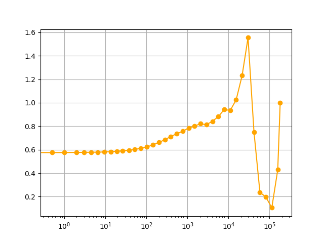
Will the relative variance be a constant?
Empirically, the relative variance is indeed a constant not too far from $1$ (see plot below). But why is that?
Suppose that currently $W_{i1} \ge W_{i2} \ge \cdots \ge W_{im} \ge 0$, and let’s look at the relative difference between the biggest weight $W_{i1}$ and some other weight $W_{ik} > 0$, i.e.
\[
\gamma_k \ce \frac{W_{i1} - W_{ik}}{W_{i1}} = 1 - \frac{W_{ik}}{W_{i1}}.
\]
Using relative derivatives, we have
\[
\frac{\d \gamma_k}{\d t} = -\frac{\d (W_{ik}/W_{i1})}{\d t} = -\frac{W_{ik}}{W_{i1}}\p{\frac{\ds{W_{ik}}t}{W_{ik}} - \frac{\ds{W_{i1}}{t}}{W_{i1}}}.
\]
Since feature benefit is a relative force, it contributes nothing to the difference of the relative derivatives of $W_{ik}$ and $W_{i1}$, so we just have the contribution from regularization
\[
\al{
\frac{\d \gamma_k}{\d t}
&= -\frac{W_{ik}}{W_{i1}}\p{\frac{-\lambda}{W_{ik}} - \frac{-\lambda}{W_{i1}}}\\
&= \frac{\lambda W_{ik}}{W_{i1}}\p{\frac{1}{W_{ik}} - \frac{1}{W_{i1}}}\\
&= \frac{\lambda}{W_{i1}}\p{1 - \frac{W_{ik}}{W_{i1}}}\\
&= \frac{\lambda}{W_{i1}}\gamma_k.
}
\]
Note that this differential equation doesn’t involve $W_{ik}$ at all! This means that there is a single function $\gamma(t)$ defined by
\[
\left\{
\al{
\gamma(0) &= 1\\
\frac{\d \gamma}{\d t}(t) &= \frac{\lambda}{W_{i1}(t)}\gamma(t)
}
\right.
\]
such that for all $k$, as long as $W_{ik}(t) > 0$,
\[
1 - \frac{W_{ik}(t)}{W_{i1}(t)} = \gamma(t)\p{1-\frac{W_{ik}(0)}{W_{i1}(0)}}
\Rightarrow
W_{ik}(t) = \UB{W_{i1}(t)\p{1 - \gamma(t)}}_\text{doesn't depend on $k$} +\UB{\frac{\gamma(t)W_{i1}(t)}{W_{i1}(0)}}_\text{doesn't depend on $k$}W_{ik}(0).
\]
In other words, the relative spacing of the nonzero weights never change: their change between times $0$ and $t$ is a single affine transformation.
Since the relative variance is scaling-invariant, we can think of this affine transformation as a simple translation. The value of the relative variance of the remaining nonzero weights $W_{i1}(t), \ldots, W_{im'}(t)$ at some point in time must be of the following form:
- take the initial values $W_{i1}(0), \ldots, W_{im}(0)$,
- translate them left by some amount which leaves $m'$ weights positive,
- drop the values that have become $\le 0$,
- then compute the relative variance of what’s left.
In particular, the relative variance when $m'$ weights are left must lie between the relative variance of
\[
\p{W_{i1}(0)-W_{i(m'+1)}(0), W_{i2}(0)-W_{i(m'+1)}(0), \ldots, W_{im'}(0)-W_{i(m'+1)}(0)}
\]
and the relative variance of
\[
\p{W_{i1}(0)-W_{im'}(0), W_{i2}(0)-W_{im'}(0), \ldots, 0}
\]
(since these extremes have the same variance but the latter has a smaller mean).
These relative variances are functions of $m'$ and the initial value of $W_i$ only, and (when $W_i$ is made of mean-$0$ normals) they will be $\Theta(1)$ with high probability in $m'$. The plot below shows these lower and upper values for $W_i(0)$ itself (in red) and for an idealized version of $W_i(0)$ that hits regular percentiles (in pink, dashed).
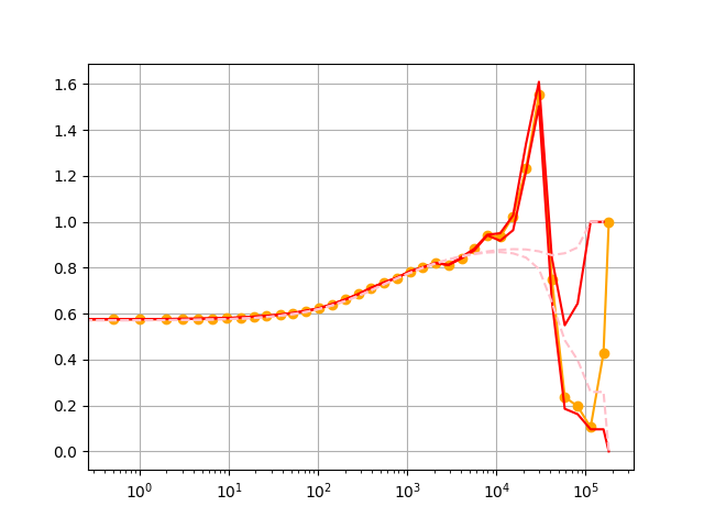
We can see that the orange curve does indeed lie within the red curves, and that the red and pink curves only start to diverge significantly at later time steps when $m'$ is smaller.