$\require{mathtools}
\newcommand{\nc}{\newcommand}
%
%%% GENERIC MATH %%%
%
% Environments
\newcommand{\al}[1]{\begin{align}#1\end{align}} % need this for \tag{} to work
\renewcommand{\r}{\mathrm} % BAD!! does cursed things with accents :((
\renewcommand{\t}{\textrm}
\newcommand{\either}[1]{\begin{cases}#1\end{cases}}
%
% Delimiters
% (I needed to create my own because the MathJax version of \DeclarePairedDelimiter doesn't have \mathopen{} and that messes up the spacing)
% .. one-part
\newcommand{\p}[1]{\mathopen{}\left( #1 \right)}
\renewcommand{\P}[1]{^{\p{#1}}}
\renewcommand{\b}[1]{\mathopen{}\left[ #1 \right]}
\newcommand{\lopen}[1]{\mathopen{}\left( #1 \right]}
\newcommand{\ropen}[1]{\mathopen{}\left[ #1 \right)}
\newcommand{\set}[1]{\mathopen{}\left\{ #1 \right\}}
\newcommand{\abs}[1]{\mathopen{}\left\lvert #1 \right\rvert}
\newcommand{\floor}[1]{\mathopen{}\left\lfloor #1 \right\rfloor}
\newcommand{\ceil}[1]{\mathopen{}\left\lceil #1 \right\rceil}
\newcommand{\round}[1]{\mathopen{}\left\lfloor #1 \right\rceil}
\newcommand{\inner}[1]{\mathopen{}\left\langle #1 \right\rangle}
\newcommand{\norm}[1]{\mathopen{}\left\lVert #1 \strut \right\rVert}
\newcommand{\frob}[1]{\norm{#1}_\mathrm{F}}
\newcommand{\mix}[1]{\mathopen{}\left\lfloor #1 \right\rceil}
%% .. two-part
\newcommand{\inco}[2]{#1 \mathop{}\middle|\mathop{} #2}
\newcommand{\co}[2]{ {\left.\inco{#1}{#2}\right.}}
\newcommand{\cond}{\co} % deprecated
\newcommand{\pco}[2]{\p{\inco{#1}{#2}}}
\newcommand{\bco}[2]{\b{\inco{#1}{#2}}}
\newcommand{\setco}[2]{\set{\inco{#1}{#2}}}
\newcommand{\at}[2]{ {\left.#1\strut\right|_{#2}}}
\newcommand{\pat}[2]{\p{\at{#1}{#2}}}
\newcommand{\bat}[2]{\b{\at{#1}{#2}}}
\newcommand{\para}[2]{#1\strut \mathop{}\middle\|\mathop{} #2}
\newcommand{\ppa}[2]{\p{\para{#1}{#2}}}
\newcommand{\pff}[2]{\p{\ff{#1}{#2}}}
\newcommand{\bff}[2]{\b{\ff{#1}{#2}}}
\newcommand{\bffco}[4]{\bff{\cond{#1}{#2}}{\cond{#3}{#4}}}
\newcommand{\sm}[1]{\p{\begin{smallmatrix}#1\end{smallmatrix}}}
%
% Greek
\newcommand{\eps}{\epsilon}
\newcommand{\veps}{\varepsilon}
\newcommand{\vpi}{\varpi}
% the following cause issues with real LaTeX tho :/ maybe consider naming it \fhi instead?
\let\fi\phi % because it looks like an f
\let\phi\varphi % because it looks like a p
\renewcommand{\th}{\theta}
\newcommand{\Th}{\Theta}
\newcommand{\om}{\omega}
\newcommand{\Om}{\Omega}
%
% Miscellaneous
\newcommand{\LHS}{\mathrm{LHS}}
\newcommand{\RHS}{\mathrm{RHS}}
\DeclareMathOperator{\cst}{const}
% .. operators
\DeclareMathOperator{\poly}{poly}
\DeclareMathOperator{\polylog}{polylog}
\DeclareMathOperator{\quasipoly}{quasipoly}
\DeclareMathOperator{\negl}{negl}
\DeclareMathOperator*{\argmin}{arg\thinspace min}
\DeclareMathOperator*{\argmax}{arg\thinspace max}
\DeclareMathOperator{\diag}{diag}
% .. functions
\DeclareMathOperator{\id}{id}
\DeclareMathOperator{\sign}{sign}
\DeclareMathOperator{\step}{step}
\DeclareMathOperator{\err}{err}
\DeclareMathOperator{\ReLU}{ReLU}
\DeclareMathOperator{\softmax}{softmax}
% .. analysis
\let\d\undefined
\newcommand{\d}{\operatorname{d}\mathopen{}}
\newcommand{\dd}[1]{\operatorname{d}^{#1}\mathopen{}}
\newcommand{\df}[2]{ {\f{\d #1}{\d #2}}}
\newcommand{\ds}[2]{ {\sl{\d #1}{\d #2}}}
\newcommand{\ddf}[3]{ {\f{\dd{#1} #2}{\p{\d #3}^{#1}}}}
\newcommand{\dds}[3]{ {\sl{\dd{#1} #2}{\p{\d #3}^{#1}}}}
\renewcommand{\part}{\partial}
\newcommand{\ppart}[1]{\part^{#1}}
\newcommand{\partf}[2]{\f{\part #1}{\part #2}}
\newcommand{\parts}[2]{\sl{\part #1}{\part #2}}
\newcommand{\ppartf}[3]{ {\f{\ppart{#1} #2}{\p{\part #3}^{#1}}}}
\newcommand{\pparts}[3]{ {\sl{\ppart{#1} #2}{\p{\part #3}^{#1}}}}
\newcommand{\grad}[1]{\mathop{\nabla\!_{#1}}}
% .. sets
\newcommand{\es}{\emptyset}
\newcommand{\N}{\mathbb{N}}
\newcommand{\Z}{\mathbb{Z}}
\newcommand{\R}{\mathbb{R}}
\newcommand{\Rge}{\R_{\ge 0}}
\newcommand{\Rgt}{\R_{> 0}}
\newcommand{\C}{\mathbb{C}}
\newcommand{\F}{\mathbb{F}}
\newcommand{\zo}{\set{0,1}}
\newcommand{\pmo}{\set{\pm 1}}
\newcommand{\zpmo}{\set{0,\pm 1}}
% .... set operations
\newcommand{\sse}{\subseteq}
\newcommand{\out}{\not\in}
\newcommand{\minus}{\setminus}
\newcommand{\inc}[1]{\union \set{#1}} % "including"
\newcommand{\exc}[1]{\setminus \set{#1}} % "except"
% .. over and under
\renewcommand{\ss}[1]{_{\substack{#1}}}
\newcommand{\OB}{\overbrace}
\newcommand{\ob}[2]{\OB{#1}^\t{#2}}
\newcommand{\UB}{\underbrace}
\newcommand{\ub}[2]{\UB{#1}_\t{#2}}
\newcommand{\ol}{\overline}
\newcommand{\tld}{\widetilde} % deprecated
\renewcommand{\~}{\widetilde}
\newcommand{\HAT}{\widehat} % deprecated
\renewcommand{\^}{\widehat}
\newcommand{\rt}[1]{ {\sqrt{#1}}}
\newcommand{\for}[2]{_{#1=1}^{#2}}
\newcommand{\sfor}{\sum\for}
\newcommand{\pfor}{\prod\for}
% .... two-part
\newcommand{\f}{\frac}
\renewcommand{\sl}[2]{#1 /\mathopen{}#2}
\newcommand{\ff}[2]{\mathchoice{\begin{smallmatrix}\displaystyle\vphantom{\p{#1}}#1\\[-0.05em]\hline\\[-0.05em]\hline\displaystyle\vphantom{\p{#2}}#2\end{smallmatrix}}{\begin{smallmatrix}\vphantom{\p{#1}}#1\\[-0.1em]\hline\\[-0.1em]\hline\vphantom{\p{#2}}#2\end{smallmatrix}}{\begin{smallmatrix}\vphantom{\p{#1}}#1\\[-0.1em]\hline\\[-0.1em]\hline\vphantom{\p{#2}}#2\end{smallmatrix}}{\begin{smallmatrix}\vphantom{\p{#1}}#1\\[-0.1em]\hline\\[-0.1em]\hline\vphantom{\p{#2}}#2\end{smallmatrix}}}
% .. arrows
\newcommand{\from}{\leftarrow}
\DeclareMathOperator*{\<}{\!\;\longleftarrow\;\!}
\let\>\undefined
\DeclareMathOperator*{\>}{\!\;\longrightarrow\;\!}
\let\-\undefined
\DeclareMathOperator*{\-}{\!\;\longleftrightarrow\;\!}
\newcommand{\so}{\implies}
% .. operators and relations
\renewcommand{\*}{\cdot}
\newcommand{\x}{\times}
\newcommand{\ox}{\otimes}
\newcommand{\OX}[1]{^{\ox #1}}
\newcommand{\sr}{\stackrel}
\newcommand{\ce}{\coloneqq}
\newcommand{\ec}{\eqqcolon}
\newcommand{\ap}{\approx}
\newcommand{\ls}{\lesssim}
\newcommand{\gs}{\gtrsim}
% .. punctuation and spacing
\renewcommand{\.}[1]{#1\dots#1}
\newcommand{\ts}{\thinspace}
\newcommand{\q}{\quad}
\newcommand{\qq}{\qquad}
%
%
%%% SPECIALIZED MATH %%%
%
% Logic and bit operations
\newcommand{\fa}{\forall}
\newcommand{\ex}{\exists}
\renewcommand{\and}{\wedge}
\newcommand{\AND}{\bigwedge}
\renewcommand{\or}{\vee}
\newcommand{\OR}{\bigvee}
\newcommand{\xor}{\oplus}
\newcommand{\XOR}{\bigoplus}
\newcommand{\union}{\cup}
\newcommand{\dunion}{\sqcup}
\newcommand{\inter}{\cap}
\newcommand{\UNION}{\bigcup}
\newcommand{\DUNION}{\bigsqcup}
\newcommand{\INTER}{\bigcap}
\newcommand{\comp}{\overline}
\newcommand{\true}{\r{true}}
\newcommand{\false}{\r{false}}
\newcommand{\tf}{\set{\true,\false}}
\DeclareMathOperator{\One}{\mathbb{1}}
\DeclareMathOperator{\1}{\mathbb{1}} % use \mathbbm instead if using real LaTeX
\DeclareMathOperator{\LSB}{LSB}
%
% Linear algebra
\newcommand{\spn}{\mathrm{span}} % do NOT use \span because it causes misery with amsmath
\DeclareMathOperator{\rank}{rank}
\DeclareMathOperator{\proj}{proj}
\DeclareMathOperator{\dom}{dom}
\DeclareMathOperator{\Img}{Im}
\DeclareMathOperator{\tr}{tr}
\DeclareMathOperator{\perm}{perm}
\DeclareMathOperator{\haf}{haf}
\newcommand{\transp}{\mathsf{T}}
\newcommand{\T}{^\transp}
\newcommand{\par}{\parallel}
% .. named tensors
\newcommand{\namedtensorstrut}{\vphantom{fg}} % milder than \mathstrut
\newcommand{\name}[1]{\mathsf{\namedtensorstrut #1}}
\newcommand{\nbin}[2]{\mathbin{\underset{\substack{#1}}{\namedtensorstrut #2}}}
\newcommand{\ndot}[1]{\nbin{#1}{\odot}}
\newcommand{\ncat}[1]{\nbin{#1}{\oplus}}
\newcommand{\nsum}[1]{\sum\limits_{\substack{#1}}}
\newcommand{\nfun}[2]{\mathop{\underset{\substack{#1}}{\namedtensorstrut\mathrm{#2}}}}
\newcommand{\ndef}[2]{\newcommand{#1}{\name{#2}}}
\newcommand{\nt}[1]{^{\transp(#1)}}
%
% Probability
\newcommand{\tri}{\triangle}
\newcommand{\Normal}{\mathcal{N}}
\newcommand{\Exp}{\mathcal{Exp}}
% .. operators
\DeclareMathOperator{\supp}{supp}
\let\Pr\undefined
\DeclareMathOperator*{\Pr}{Pr}
\DeclareMathOperator*{\G}{\mathbb{G}}
\DeclareMathOperator*{\Odds}{Od}
\DeclareMathOperator*{\E}{E}
\DeclareMathOperator*{\Var}{Var}
\DeclareMathOperator*{\Cov}{Cov}
\DeclareMathOperator*{\K}{K}
\DeclareMathOperator*{\corr}{corr}
\DeclareMathOperator*{\median}{median}
\DeclareMathOperator*{\maj}{maj}
% ... information theory
\let\H\undefined
\DeclareMathOperator*{\H}{H}
\DeclareMathOperator*{\I}{I}
\DeclareMathOperator*{\D}{D}
\DeclareMathOperator*{\KL}{KL}
% .. other divergences
\newcommand{\dTV}{d_{\mathrm{TV}}}
\newcommand{\dHel}{d_{\mathrm{Hel}}}
\newcommand{\dJS}{d_{\mathrm{JS}}}
%
% Polynomials
\DeclareMathOperator{\He}{He}
\DeclareMathOperator{\coeff}{coeff}
%
%%% SPECIALIZED COMPUTER SCIENCE %%%
%
% Complexity classes
% .. keywords
\newcommand{\coclass}{\mathsf{co}}
\newcommand{\Prom}{\mathsf{Promise}}
% .. classical
\newcommand{\PTIME}{\mathsf{P}}
\newcommand{\NP}{\mathsf{NP}}
\newcommand{\coNP}{\coclass\NP}
\newcommand{\PH}{\mathsf{PH}}
\newcommand{\PSPACE}{\mathsf{PSPACE}}
\renewcommand{\L}{\mathsf{L}}
\newcommand{\EXP}{\mathsf{EXP}}
\newcommand{\NEXP}{\mathsf{NEXP}}
% .. probabilistic
\newcommand{\formost}{\mathsf{Я}}
\newcommand{\RP}{\mathsf{RP}}
\newcommand{\BPP}{\mathsf{BPP}}
\newcommand{\ZPP}{\mathsf{ZPP}}
\newcommand{\MA}{\mathsf{MA}}
\newcommand{\AM}{\mathsf{AM}}
\newcommand{\IP}{\mathsf{IP}}
\newcommand{\RL}{\mathsf{RL}}
% .. circuits
\newcommand{\NC}{\mathsf{NC}}
\newcommand{\AC}{\mathsf{AC}}
\newcommand{\ACC}{\mathsf{ACC}}
\newcommand{\ThrC}{\mathsf{TC}}
\newcommand{\Ppoly}{\mathsf{P}/\poly}
\newcommand{\Lpoly}{\mathsf{L}/\poly}
% .. resources
\newcommand{\TIME}{\mathsf{TIME}}
\newcommand{\NTIME}{\mathsf{NTIME}}
\newcommand{\SPACE}{\mathsf{SPACE}}
\newcommand{\TISP}{\mathsf{TISP}}
\newcommand{\SIZE}{\mathsf{SIZE}}
% .. custom
\newcommand{\NCP}{\mathsf{NCP}}
%
% Boolean analysis
\newcommand{\harpoon}{\!\upharpoonright\!}
\newcommand{\rr}[2]{#1\harpoon_{#2}}
\newcommand{\Fou}[1]{\widehat{#1}}
\DeclareMathOperator{\Ind}{\mathrm{Ind}}
\DeclareMathOperator{\Inf}{\mathrm{Inf}}
\newcommand{\Der}[1]{\operatorname{D}_{#1}\mathopen{}}
% \newcommand{\Exp}[1]{\operatorname{E}_{#1}\mathopen{}}
\DeclareMathOperator{\Stab}{\mathrm{Stab}}
\DeclareMathOperator{\Tau}{T}
\DeclareMathOperator{\sens}{\mathrm{s}}
\DeclareMathOperator{\bsens}{\mathrm{bs}}
\DeclareMathOperator{\fbsens}{\mathrm{fbs}}
\DeclareMathOperator{\Cert}{\mathrm{C}}
\DeclareMathOperator{\DT}{\mathrm{DT}}
\DeclareMathOperator{\CDT}{\mathrm{CDT}} % canonical
\DeclareMathOperator{\ECDT}{\mathrm{ECDT}}
\DeclareMathOperator{\CDTv}{\mathrm{CDT_{vars}}}
\DeclareMathOperator{\ECDTv}{\mathrm{ECDT_{vars}}}
\DeclareMathOperator{\CDTt}{\mathrm{CDT_{terms}}}
\DeclareMathOperator{\ECDTt}{\mathrm{ECDT_{terms}}}
\DeclareMathOperator{\CDTw}{\mathrm{CDT_{weighted}}}
\DeclareMathOperator{\ECDTw}{\mathrm{ECDT_{weighted}}}
\DeclareMathOperator{\AvgDT}{\mathrm{AvgDT}}
\DeclareMathOperator{\PDT}{\mathrm{PDT}} % partial decision tree
\DeclareMathOperator{\DTsize}{\mathrm{DT_{size}}}
\DeclareMathOperator{\W}{\mathbf{W}}
% .. functions (small caps sadly doesn't work)
\DeclareMathOperator{\Par}{\mathrm{Par}}
\DeclareMathOperator{\Maj}{\mathrm{Maj}}
\DeclareMathOperator{\HW}{\mathrm{HW}}
\DeclareMathOperator{\Thr}{\mathrm{Thr}}
\DeclareMathOperator{\Tribes}{\mathrm{Tribes}}
\DeclareMathOperator{\RotTribes}{\mathrm{RotTribes}}
\DeclareMathOperator{\CycleRun}{\mathrm{CycleRun}}
\DeclareMathOperator{\SAT}{\mathrm{SAT}}
\DeclareMathOperator{\UniqueSAT}{\mathrm{UniqueSAT}}
%
% Dynamic optimality
\newcommand{\OPT}{\mathsf{OPT}}
\newcommand{\Alt}{\mathsf{Alt}}
\newcommand{\Funnel}{\mathsf{Funnel}}
%
% Alignment
\DeclareMathOperator{\Amp}{\mathrm{Amp}}
%
%%% TYPESETTING %%%
%
% In "text"
\newcommand{\heart}{\heartsuit}
\newcommand{\nth}{^\t{th}}
\newcommand{\degree}{^\circ}
\newcommand{\qu}[1]{\text{``}#1\text{''}}
% remove these last two if using real LaTeX
\newcommand{\qed}{\blacksquare}
\newcommand{\qedhere}{\tag*{$\blacksquare$}}
%
% Fonts
% .. bold
\newcommand{\BA}{\boldsymbol{A}}
\newcommand{\BB}{\boldsymbol{B}}
\newcommand{\BC}{\boldsymbol{C}}
\newcommand{\BD}{\boldsymbol{D}}
\newcommand{\BE}{\boldsymbol{E}}
\newcommand{\BF}{\boldsymbol{F}}
\newcommand{\BG}{\boldsymbol{G}}
\newcommand{\BH}{\boldsymbol{H}}
\newcommand{\BI}{\boldsymbol{I}}
\newcommand{\BJ}{\boldsymbol{J}}
\newcommand{\BK}{\boldsymbol{K}}
\newcommand{\BL}{\boldsymbol{L}}
\newcommand{\BM}{\boldsymbol{M}}
\newcommand{\BN}{\boldsymbol{N}}
\newcommand{\BO}{\boldsymbol{O}}
\newcommand{\BP}{\boldsymbol{P}}
\newcommand{\BQ}{\boldsymbol{Q}}
\newcommand{\BR}{\boldsymbol{R}}
\newcommand{\BS}{\boldsymbol{S}}
\newcommand{\BT}{\boldsymbol{T}}
\newcommand{\BU}{\boldsymbol{U}}
\newcommand{\BV}{\boldsymbol{V}}
\newcommand{\BW}{\boldsymbol{W}}
\newcommand{\BX}{\boldsymbol{X}}
\newcommand{\BY}{\boldsymbol{Y}}
\newcommand{\BZ}{\boldsymbol{Z}}
\newcommand{\Ba}{\boldsymbol{a}}
\newcommand{\Bb}{\boldsymbol{b}}
\newcommand{\Bc}{\boldsymbol{c}}
\newcommand{\Bd}{\boldsymbol{d}}
\newcommand{\Be}{\boldsymbol{e}}
\newcommand{\Bf}{\boldsymbol{f}}
\newcommand{\Bg}{\boldsymbol{g}}
\newcommand{\Bh}{\boldsymbol{h}}
\newcommand{\Bi}{\boldsymbol{i}}
\newcommand{\Bj}{\boldsymbol{j}}
\newcommand{\Bk}{\boldsymbol{k}}
\newcommand{\Bl}{\boldsymbol{l}}
\newcommand{\Bm}{\boldsymbol{m}}
\newcommand{\Bn}{\boldsymbol{n}}
\newcommand{\Bo}{\boldsymbol{o}}
\newcommand{\Bp}{\boldsymbol{p}}
\newcommand{\Bq}{\boldsymbol{q}}
\newcommand{\Br}{\boldsymbol{r}}
\newcommand{\Bs}{\boldsymbol{s}}
\newcommand{\Bt}{\boldsymbol{t}}
\newcommand{\Bu}{\boldsymbol{u}}
\newcommand{\Bv}{\boldsymbol{v}}
\newcommand{\Bw}{\boldsymbol{w}}
\newcommand{\Bx}{\boldsymbol{x}}
\newcommand{\By}{\boldsymbol{y}}
\newcommand{\Bz}{\boldsymbol{z}}
\newcommand{\Balpha}{\boldsymbol{\alpha}}
\newcommand{\Bbeta}{\boldsymbol{\beta}}
\newcommand{\Bgamma}{\boldsymbol{\gamma}}
\newcommand{\Bdelta}{\boldsymbol{\delta}}
\newcommand{\Beps}{\boldsymbol{\eps}}
\newcommand{\Bveps}{\boldsymbol{\veps}}
\newcommand{\Bzeta}{\boldsymbol{\zeta}}
\newcommand{\Beta}{\boldsymbol{\eta}}
\newcommand{\Btheta}{\boldsymbol{\theta}}
\newcommand{\Bth}{\boldsymbol{\th}}
\newcommand{\Biota}{\boldsymbol{\iota}}
\newcommand{\Bkappa}{\boldsymbol{\kappa}}
\newcommand{\Blambda}{\boldsymbol{\lambda}}
\newcommand{\Bmu}{\boldsymbol{\mu}}
\newcommand{\Bnu}{\boldsymbol{\nu}}
\newcommand{\Bxi}{\boldsymbol{\xi}}
\newcommand{\Bpi}{\boldsymbol{\pi}}
\newcommand{\Bvpi}{\boldsymbol{\vpi}}
\newcommand{\Brho}{\boldsymbol{\rho}}
\newcommand{\Bsigma}{\boldsymbol{\sigma}}
\newcommand{\Btau}{\boldsymbol{\tau}}
\newcommand{\Bupsilon}{\boldsymbol{\upsilon}}
\newcommand{\Bphi}{\boldsymbol{\phi}}
\newcommand{\Bfi}{\boldsymbol{\fi}}
\newcommand{\Bchi}{\boldsymbol{\chi}}
\newcommand{\Bpsi}{\boldsymbol{\psi}}
\newcommand{\Bom}{\boldsymbol{\om}}
% .. calligraphic
\newcommand{\CA}{\mathcal{A}}
\newcommand{\CB}{\mathcal{B}}
\newcommand{\CC}{\mathcal{C}}
\newcommand{\CD}{\mathcal{D}}
\newcommand{\CE}{\mathcal{E}}
\newcommand{\CF}{\mathcal{F}}
\newcommand{\CG}{\mathcal{G}}
\newcommand{\CH}{\mathcal{H}}
\newcommand{\CI}{\mathcal{I}}
\newcommand{\CJ}{\mathcal{J}}
\newcommand{\CK}{\mathcal{K}}
\newcommand{\CL}{\mathcal{L}}
\newcommand{\CM}{\mathcal{M}}
\newcommand{\CN}{\mathcal{N}}
\newcommand{\CO}{\mathcal{O}}
\newcommand{\CP}{\mathcal{P}}
\newcommand{\CQ}{\mathcal{Q}}
\newcommand{\CR}{\mathcal{R}}
\newcommand{\CS}{\mathcal{S}}
\newcommand{\CT}{\mathcal{T}}
\newcommand{\CU}{\mathcal{U}}
\newcommand{\CV}{\mathcal{V}}
\newcommand{\CW}{\mathcal{W}}
\newcommand{\CX}{\mathcal{X}}
\newcommand{\CY}{\mathcal{Y}}
\newcommand{\CZ}{\mathcal{Z}}
% .. typewriter
\newcommand{\TA}{\mathtt{A}}
\newcommand{\TB}{\mathtt{B}}
\newcommand{\TC}{\mathtt{C}}
\newcommand{\TD}{\mathtt{D}}
\newcommand{\TE}{\mathtt{E}}
\newcommand{\TF}{\mathtt{F}}
\newcommand{\TG}{\mathtt{G}}
\renewcommand{\TH}{\mathtt{H}}
\newcommand{\TI}{\mathtt{I}}
\newcommand{\TJ}{\mathtt{J}}
\newcommand{\TK}{\mathtt{K}}
\newcommand{\TL}{\mathtt{L}}
\newcommand{\TM}{\mathtt{M}}
\newcommand{\TN}{\mathtt{N}}
\newcommand{\TO}{\mathtt{O}}
\newcommand{\TP}{\mathtt{P}}
\newcommand{\TQ}{\mathtt{Q}}
\newcommand{\TR}{\mathtt{R}}
\newcommand{\TS}{\mathtt{S}}
\newcommand{\TT}{\mathtt{T}}
\newcommand{\TU}{\mathtt{U}}
\newcommand{\TV}{\mathtt{V}}
\newcommand{\TW}{\mathtt{W}}
\newcommand{\TX}{\mathtt{X}}
\newcommand{\TY}{\mathtt{Y}}
\newcommand{\TZ}{\mathtt{Z}}
%
% LEVELS OF CLOSENESS (basically deprecated)
\newcommand{\scirc}[1]{\sr{\circ}{#1}}
\newcommand{\sdot}[1]{\sr{.}{#1}}
\newcommand{\slog}[1]{\sr{\log}{#1}}
\newcommand{\createClosenessLevels}[7]{
\newcommand{#2}{\mathrel{(#1)}}
\newcommand{#3}{\mathrel{#1}}
\newcommand{#4}{\mathrel{#1\!\!#1}}
\newcommand{#5}{\mathrel{#1\!\!#1\!\!#1}}
\newcommand{#6}{\mathrel{(\sdot{#1})}}
\newcommand{#7}{\mathrel{(\slog{#1})}}
}
\let\lt\undefined
\let\gt\undefined
% .. vanilla versions (is it within a constant?)
\newcommand{\ez}{\scirc=}
\newcommand{\eq}{\simeq}
\newcommand{\eqq}{\mathrel{\eq\!\!\eq}}
\newcommand{\eqqq}{\mathrel{\eq\!\!\eq\!\!\eq}}
\newcommand{\lez}{\scirc\le}
\renewcommand{\lq}{\preceq}
\newcommand{\lqq}{\mathrel{\lq\!\!\lq}}
\newcommand{\lqqq}{\mathrel{\lq\!\!\lq\!\!\lq}}
\newcommand{\gez}{\scirc\ge}
\newcommand{\gq}{\succeq}
\newcommand{\gqq}{\mathrel{\gq\!\!\gq}}
\newcommand{\gqqq}{\mathrel{\gq\!\!\gq\!\!\gq}}
\newcommand{\lz}{\scirc<}
\newcommand{\lt}{\prec}
\newcommand{\ltt}{\mathrel{\lt\!\!\lt}}
\newcommand{\lttt}{\mathrel{\lt\!\!\lt\!\!\lt}}
\newcommand{\gz}{\scirc>}
\newcommand{\gt}{\succ}
\newcommand{\gtt}{\mathrel{\gt\!\!\gt}}
\newcommand{\gttt}{\mathrel{\gt\!\!\gt\!\!\gt}}
% .. dotted versions (is it equal in the limit?)
\newcommand{\ed}{\sdot=}
\newcommand{\eqd}{\sdot\eq}
\newcommand{\eqqd}{\sdot\eqq}
\newcommand{\eqqqd}{\sdot\eqqq}
\newcommand{\led}{\sdot\le}
\newcommand{\lqd}{\sdot\lq}
\newcommand{\lqqd}{\sdot\lqq}
\newcommand{\lqqqd}{\sdot\lqqq}
\newcommand{\ged}{\sdot\ge}
\newcommand{\gqd}{\sdot\gq}
\newcommand{\gqqd}{\sdot\gqq}
\newcommand{\gqqqd}{\sdot\gqqq}
\newcommand{\ld}{\sdot<}
\newcommand{\ltd}{\sdot\lt}
\newcommand{\lttd}{\sdot\ltt}
\newcommand{\ltttd}{\sdot\lttt}
\newcommand{\gd}{\sdot>}
\newcommand{\gtd}{\sdot\gt}
\newcommand{\gttd}{\sdot\gtt}
\newcommand{\gtttd}{\sdot\gttt}
% .. log versions (is it equal up to log?)
\newcommand{\elog}{\slog=}
\newcommand{\eqlog}{\slog\eq}
\newcommand{\eqqlog}{\slog\eqq}
\newcommand{\eqqqlog}{\slog\eqqq}
\newcommand{\lelog}{\slog\le}
\newcommand{\lqlog}{\slog\lq}
\newcommand{\lqqlog}{\slog\lqq}
\newcommand{\lqqqlog}{\slog\lqqq}
\newcommand{\gelog}{\slog\ge}
\newcommand{\gqlog}{\slog\gq}
\newcommand{\gqqlog}{\slog\gqq}
\newcommand{\gqqqlog}{\slog\gqqq}
\newcommand{\llog}{\slog<}
\newcommand{\ltlog}{\slog\lt}
\newcommand{\lttlog}{\slog\ltt}
\newcommand{\ltttlog}{\slog\lttt}
\newcommand{\glog}{\slog>}
\newcommand{\gtlog}{\slog\gt}
\newcommand{\gttlog}{\slog\gtt}
\newcommand{\gtttlog}{\slog\gttt}$
Adapted from a great talk by Erik Waingarten at the teach-us-anything seminar at Stanford.
Problem and linear program
Given a weighted $K_{n \times n}$ (with non-negative weights), find a perfect matching of minimum total cost.
We can express it as the following linear program:
minimize $\sum_{i,j} c_{i,j} x_{i,j}$ subject to
- $x_{i,j} \geq 0$
- $\sum_j x_{i,j} = 1$ (flow 1 from left)
- $\sum_i x_{i,j} = 1$ (flow 1 to right)
But in fact it’s easy to see we can rephrase the constraints in a “supply-and-demand” style without modifying the space of solutions:
minimize $\sum_{i,j} c_{i,j} x_{i,j}$ subject to
- $x_{i,j} \geq 0$
- $\sum_j x_{i,j} \leq 1$ (left can supply at most 1 unit)
- $\sum_i x_{i,j} \geq 1$ (right demands at least 1 unit)
This is because if each right vertex “demands” 1 unit of flow, overall $n$ units of flow must be provided, so if even one left vertex slacks off, not enough flow is provided.
Duality
Now, an alternate way to express constraints is as a two-player game between a minimizer (us) and an maximizer (the adversary). To make sure we’re incentivized to satisfy the constraints, we can let an adversary penalize us to infinity when we violate them.
\[\min_{x_{i,j} \geq 0} \max_{\alpha_i, \beta_j \geq 0} \sum_{i,j} c_{i,j}x_{i,j} + \sum_i\alpha_i\left(\sum_j x_{i,j} - 1\right) + \sum_j\beta_j \left(1 - \sum_i x_{i,j}\right)\]
Right now, the adversary has a lot of power because it is allowed to pick $\alpha_i, \beta_j$ after we’ve committed to our values $x_{i,j}$. On the other hand, if we switched the $\min$ and the $\max$, we (the minimizers) would have the adaptivity: we could adapt $x_{i,j}$ to their choice of $\alpha_i, \beta_j$, which the adversary would have to make in advance. So we can only do a better job, and the value can only decrease. This is called weak duality.
\[\max_{\alpha_i, \beta_j \geq 0} \min_{x_{i,j} \geq 0} \sum_{i,j} c_{i,j}x_{i,j} + \sum_i\alpha_i\left(\sum_j x_{i,j} - 1\right) + \sum_j\beta_j \left(1 - \sum_i x_{i,j}\right)\]
Let’s rearrange a bit to make it clear what role $x_{i,j}$ plays when $\alpha_i, \beta_j$ are fixed.
\[\max_{\alpha_i, \beta_j \geq 0} \min_{x_{i,j} \geq 0} \sum_j\beta_j - \sum_i\alpha_i + \sum_{i,j} x_{i,j}(c_{i,j} + \alpha_i - \beta_j)\]
Finally, we can do the first transformation in reverse: since we can pick any non-negative value for $x_{i,j}$, in order to minimize the expression, it makes sense to make it arbitrarily high when $c_{i,j} + \alpha_i - \beta_j < 0$ (and keep it at $0$ when $c_{i,j} + \alpha_i - \beta_j \geq 0$). So the adversary is being arbitrarily penalized whenever it lets $c_{i,j} + \alpha_i - \beta_j$ be negative. Therefore, it will work as if $c_{i,j} + \alpha_i - \beta_j \geq 0$ were a constraint. So the max-min problem above is equivalent to the following dual LP:
maximize $\sum_j \beta_j - \sum_i \alpha_i$ subject to
- $\alpha_i, \beta_j \geq 0$
- $\beta_j - \alpha_i \leq c_{i,j}$ (“$\beta_j$ is at most $c_{i,j}$ units to the right of $\alpha_i$”)
We’ve shown that the optimum of this dual is upper bounded by the optimum of the original problem (the primal). Also, the primal was a minimization while dual is maximization. So dual solutions are lower bounds on the primal, and the better they are, the better the lower bound. A priori, there might be a “gap” between the possible values for the primal and the dual. But if there is no gap and we can somehow find a primal solution and a dual solution whose values match, then they must both be optimal!
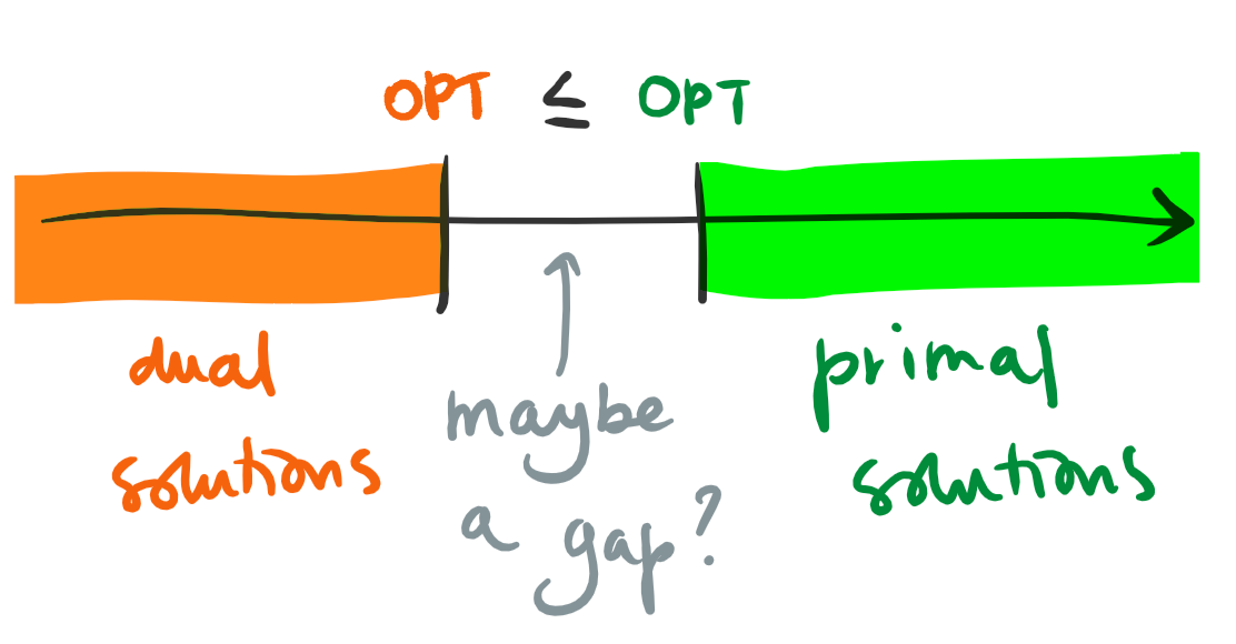
The primal-dual method is a way to use that idea in algorithms. The algorithm starts out with a valid dual solution, and an invalid primal solution of the same value. It then progressively modifies both (while keeping them at equal values) until the primal constraints are satisfied. Once that happens, we know the solution is optimal.
The algorithm
Taking a closer look at the dual:
- we have numbers $\alpha_i$ for each vertex on the left and $\beta_j$ for each vertex on the left;
- we want to pull the $\beta_j$’s as far as possible to the right and the $\alpha_i$’s as far as possible to the left;
- but $\beta_j$ cannot go more than $c_{i,j}$ distance to the right of $\alpha_i$: it’s as if points $\alpha_i$ and $\beta_j$ were connected by a string of length $c_{i,j}$.
Based on this analogy, the algorithm will maintain a matching and some points $\alpha_i, \beta_j$ on the number line. For $j \in \set{1, \ldots, n}$, do the following:
- “Pull” on $\beta_j$ until a string from some $\alpha_i$ gets taut.
- If the corresponding $i$ is already matched to some $j'$, start pulling both $\alpha_i$ and $\beta_{j'}$ along with $\beta_j$ (as if a solid rod was placed between $\alpha_i$ and $\beta_{j'}$) then go back to step 1.
- Otherwise, the sequence of taut strings and rods will form an augmenting path (taut strings = unmatched, rods = matched). Use it to augment the matching: set $x_{ij} \gets 1$, $x_{ij'}\gets 0$, $x_{i'j'} \gets 1$, etc.
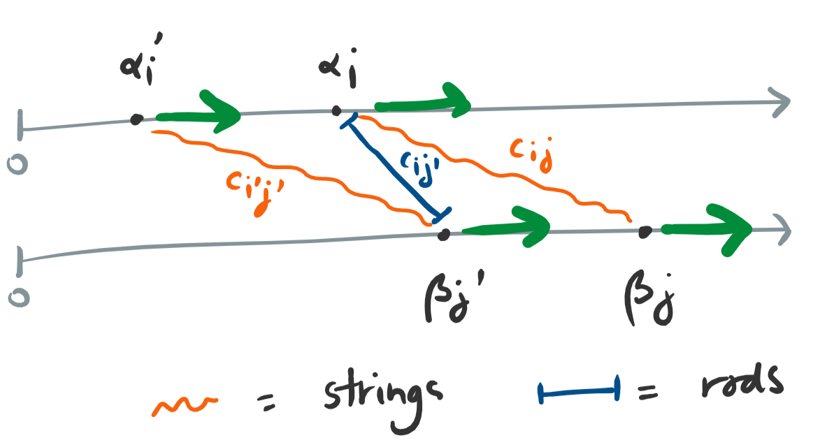
(in the picture, the axes for the $\alpha$’s and the $\beta$’s are drawn some distance apart for clarity, but you should imagine them coinciding)
One can easily verify that:
- At the start of any step, unmatched vertices have the corresponding $\alpha_i$ or $\beta_j$ set to $0$ (in particular, at the start of the $j\nth$ step, $\beta_j=0$). On the other hand, if $i,j$ are matched together, then $\beta_j - \alpha_i = c_{ij}$.
- At any time, we’re pulling exactly one more $\beta$ than we’re pulling $\alpha$’s. So during step $j$ the dual will increase by the value $\beta_j$ gets at the end of the step.
- By cancellation, the primal objective will increase by that same value.
Therefore, by the end of the algorithm, the primal and dual objective will have the same value, and the constraints of both will be satisfied: we’re satisfying the primal conditions because we built a matching, and we were satisfying the dual conditions all along by not breaking the strings. So the solution is optimal!
Each iteration takes $O(n^2)$ time (it’s basically a DFS), and there are $n$ iterations, so this takes $O(n^3)$ time overall.