$\require{mathtools}
\newcommand{\nc}{\newcommand}
%
%%% GENERIC MATH %%%
%
% Environments
\newcommand{\al}[1]{\begin{align}#1\end{align}} % need this for \tag{} to work
\renewcommand{\r}{\mathrm} % BAD!! does cursed things with accents :((
\renewcommand{\t}{\textrm}
\newcommand{\either}[1]{\begin{cases}#1\end{cases}}
%
% Delimiters
% (I needed to create my own because the MathJax version of \DeclarePairedDelimiter doesn't have \mathopen{} and that messes up the spacing)
% .. one-part
\newcommand{\p}[1]{\mathopen{}\left( #1 \right)}
\renewcommand{\P}[1]{^{\p{#1}}}
\renewcommand{\b}[1]{\mathopen{}\left[ #1 \right]}
\newcommand{\lopen}[1]{\mathopen{}\left( #1 \right]}
\newcommand{\ropen}[1]{\mathopen{}\left[ #1 \right)}
\newcommand{\set}[1]{\mathopen{}\left\{ #1 \right\}}
\newcommand{\abs}[1]{\mathopen{}\left\lvert #1 \right\rvert}
\newcommand{\floor}[1]{\mathopen{}\left\lfloor #1 \right\rfloor}
\newcommand{\ceil}[1]{\mathopen{}\left\lceil #1 \right\rceil}
\newcommand{\round}[1]{\mathopen{}\left\lfloor #1 \right\rceil}
\newcommand{\inner}[1]{\mathopen{}\left\langle #1 \right\rangle}
\newcommand{\norm}[1]{\mathopen{}\left\lVert #1 \strut \right\rVert}
\newcommand{\frob}[1]{\norm{#1}_\mathrm{F}}
\newcommand{\mix}[1]{\mathopen{}\left\lfloor #1 \right\rceil}
%% .. two-part
\newcommand{\inco}[2]{#1 \mathop{}\middle|\mathop{} #2}
\newcommand{\co}[2]{ {\left.\inco{#1}{#2}\right.}}
\newcommand{\cond}{\co} % deprecated
\newcommand{\pco}[2]{\p{\inco{#1}{#2}}}
\newcommand{\bco}[2]{\b{\inco{#1}{#2}}}
\newcommand{\setco}[2]{\set{\inco{#1}{#2}}}
\newcommand{\at}[2]{ {\left.#1\strut\right|_{#2}}}
\newcommand{\pat}[2]{\p{\at{#1}{#2}}}
\newcommand{\bat}[2]{\b{\at{#1}{#2}}}
\newcommand{\para}[2]{#1\strut \mathop{}\middle\|\mathop{} #2}
\newcommand{\ppa}[2]{\p{\para{#1}{#2}}}
\newcommand{\pff}[2]{\p{\ff{#1}{#2}}}
\newcommand{\bff}[2]{\b{\ff{#1}{#2}}}
\newcommand{\bffco}[4]{\bff{\cond{#1}{#2}}{\cond{#3}{#4}}}
\newcommand{\sm}[1]{\p{\begin{smallmatrix}#1\end{smallmatrix}}}
%
% Greek
\newcommand{\eps}{\epsilon}
\newcommand{\veps}{\varepsilon}
\newcommand{\vpi}{\varpi}
% the following cause issues with real LaTeX tho :/ maybe consider naming it \fhi instead?
\let\fi\phi % because it looks like an f
\let\phi\varphi % because it looks like a p
\renewcommand{\th}{\theta}
\newcommand{\Th}{\Theta}
\newcommand{\om}{\omega}
\newcommand{\Om}{\Omega}
%
% Miscellaneous
\newcommand{\LHS}{\mathrm{LHS}}
\newcommand{\RHS}{\mathrm{RHS}}
\DeclareMathOperator{\cst}{const}
% .. operators
\DeclareMathOperator{\poly}{poly}
\DeclareMathOperator{\polylog}{polylog}
\DeclareMathOperator{\quasipoly}{quasipoly}
\DeclareMathOperator{\negl}{negl}
\DeclareMathOperator*{\argmin}{arg\thinspace min}
\DeclareMathOperator*{\argmax}{arg\thinspace max}
\DeclareMathOperator{\diag}{diag}
% .. functions
\DeclareMathOperator{\id}{id}
\DeclareMathOperator{\sign}{sign}
\DeclareMathOperator{\step}{step}
\DeclareMathOperator{\err}{err}
\DeclareMathOperator{\ReLU}{ReLU}
\DeclareMathOperator{\softmax}{softmax}
% .. analysis
\let\d\undefined
\newcommand{\d}{\operatorname{d}\mathopen{}}
\newcommand{\dd}[1]{\operatorname{d}^{#1}\mathopen{}}
\newcommand{\df}[2]{ {\f{\d #1}{\d #2}}}
\newcommand{\ds}[2]{ {\sl{\d #1}{\d #2}}}
\newcommand{\ddf}[3]{ {\f{\dd{#1} #2}{\p{\d #3}^{#1}}}}
\newcommand{\dds}[3]{ {\sl{\dd{#1} #2}{\p{\d #3}^{#1}}}}
\renewcommand{\part}{\partial}
\newcommand{\ppart}[1]{\part^{#1}}
\newcommand{\partf}[2]{\f{\part #1}{\part #2}}
\newcommand{\parts}[2]{\sl{\part #1}{\part #2}}
\newcommand{\ppartf}[3]{ {\f{\ppart{#1} #2}{\p{\part #3}^{#1}}}}
\newcommand{\pparts}[3]{ {\sl{\ppart{#1} #2}{\p{\part #3}^{#1}}}}
\newcommand{\grad}[1]{\mathop{\nabla\!_{#1}}}
% .. sets
\newcommand{\es}{\emptyset}
\newcommand{\N}{\mathbb{N}}
\newcommand{\Z}{\mathbb{Z}}
\newcommand{\R}{\mathbb{R}}
\newcommand{\Rge}{\R_{\ge 0}}
\newcommand{\Rgt}{\R_{> 0}}
\newcommand{\C}{\mathbb{C}}
\newcommand{\F}{\mathbb{F}}
\newcommand{\zo}{\set{0,1}}
\newcommand{\pmo}{\set{\pm 1}}
\newcommand{\zpmo}{\set{0,\pm 1}}
% .... set operations
\newcommand{\sse}{\subseteq}
\newcommand{\out}{\not\in}
\newcommand{\minus}{\setminus}
\newcommand{\inc}[1]{\union \set{#1}} % "including"
\newcommand{\exc}[1]{\setminus \set{#1}} % "except"
% .. over and under
\renewcommand{\ss}[1]{_{\substack{#1}}}
\newcommand{\OB}{\overbrace}
\newcommand{\ob}[2]{\OB{#1}^\t{#2}}
\newcommand{\UB}{\underbrace}
\newcommand{\ub}[2]{\UB{#1}_\t{#2}}
\newcommand{\ol}{\overline}
\newcommand{\tld}{\widetilde} % deprecated
\renewcommand{\~}{\widetilde}
\newcommand{\HAT}{\widehat} % deprecated
\renewcommand{\^}{\widehat}
\newcommand{\rt}[1]{ {\sqrt{#1}}}
\newcommand{\for}[2]{_{#1=1}^{#2}}
\newcommand{\sfor}{\sum\for}
\newcommand{\pfor}{\prod\for}
% .... two-part
\newcommand{\f}{\frac}
\renewcommand{\sl}[2]{#1 /\mathopen{}#2}
\newcommand{\ff}[2]{\mathchoice{\begin{smallmatrix}\displaystyle\vphantom{\p{#1}}#1\\[-0.05em]\hline\\[-0.05em]\hline\displaystyle\vphantom{\p{#2}}#2\end{smallmatrix}}{\begin{smallmatrix}\vphantom{\p{#1}}#1\\[-0.1em]\hline\\[-0.1em]\hline\vphantom{\p{#2}}#2\end{smallmatrix}}{\begin{smallmatrix}\vphantom{\p{#1}}#1\\[-0.1em]\hline\\[-0.1em]\hline\vphantom{\p{#2}}#2\end{smallmatrix}}{\begin{smallmatrix}\vphantom{\p{#1}}#1\\[-0.1em]\hline\\[-0.1em]\hline\vphantom{\p{#2}}#2\end{smallmatrix}}}
% .. arrows
\newcommand{\from}{\leftarrow}
\DeclareMathOperator*{\<}{\!\;\longleftarrow\;\!}
\let\>\undefined
\DeclareMathOperator*{\>}{\!\;\longrightarrow\;\!}
\let\-\undefined
\DeclareMathOperator*{\-}{\!\;\longleftrightarrow\;\!}
\newcommand{\so}{\implies}
% .. operators and relations
\renewcommand{\*}{\cdot}
\newcommand{\x}{\times}
\newcommand{\ox}{\otimes}
\newcommand{\OX}[1]{^{\ox #1}}
\newcommand{\sr}{\stackrel}
\newcommand{\ce}{\coloneqq}
\newcommand{\ec}{\eqqcolon}
\newcommand{\ap}{\approx}
\newcommand{\ls}{\lesssim}
\newcommand{\gs}{\gtrsim}
% .. punctuation and spacing
\renewcommand{\.}[1]{#1\dots#1}
\newcommand{\ts}{\thinspace}
\newcommand{\q}{\quad}
\newcommand{\qq}{\qquad}
%
%
%%% SPECIALIZED MATH %%%
%
% Logic and bit operations
\newcommand{\fa}{\forall}
\newcommand{\ex}{\exists}
\renewcommand{\and}{\wedge}
\newcommand{\AND}{\bigwedge}
\renewcommand{\or}{\vee}
\newcommand{\OR}{\bigvee}
\newcommand{\xor}{\oplus}
\newcommand{\XOR}{\bigoplus}
\newcommand{\union}{\cup}
\newcommand{\dunion}{\sqcup}
\newcommand{\inter}{\cap}
\newcommand{\UNION}{\bigcup}
\newcommand{\DUNION}{\bigsqcup}
\newcommand{\INTER}{\bigcap}
\newcommand{\comp}{\overline}
\newcommand{\true}{\r{true}}
\newcommand{\false}{\r{false}}
\newcommand{\tf}{\set{\true,\false}}
\DeclareMathOperator{\One}{\mathbb{1}}
\DeclareMathOperator{\1}{\mathbb{1}} % use \mathbbm instead if using real LaTeX
\DeclareMathOperator{\LSB}{LSB}
%
% Linear algebra
\newcommand{\spn}{\mathrm{span}} % do NOT use \span because it causes misery with amsmath
\DeclareMathOperator{\rank}{rank}
\DeclareMathOperator{\proj}{proj}
\DeclareMathOperator{\dom}{dom}
\DeclareMathOperator{\Img}{Im}
\DeclareMathOperator{\tr}{tr}
\DeclareMathOperator{\perm}{perm}
\DeclareMathOperator{\haf}{haf}
\newcommand{\transp}{\mathsf{T}}
\newcommand{\T}{^\transp}
\newcommand{\par}{\parallel}
% .. named tensors
\newcommand{\namedtensorstrut}{\vphantom{fg}} % milder than \mathstrut
\newcommand{\name}[1]{\mathsf{\namedtensorstrut #1}}
\newcommand{\nbin}[2]{\mathbin{\underset{\substack{#1}}{\namedtensorstrut #2}}}
\newcommand{\ndot}[1]{\nbin{#1}{\odot}}
\newcommand{\ncat}[1]{\nbin{#1}{\oplus}}
\newcommand{\nsum}[1]{\sum\limits_{\substack{#1}}}
\newcommand{\nfun}[2]{\mathop{\underset{\substack{#1}}{\namedtensorstrut\mathrm{#2}}}}
\newcommand{\ndef}[2]{\newcommand{#1}{\name{#2}}}
\newcommand{\nt}[1]{^{\transp(#1)}}
%
% Probability
\newcommand{\tri}{\triangle}
\newcommand{\Normal}{\mathcal{N}}
\newcommand{\Exp}{\mathcal{Exp}}
% .. operators
\DeclareMathOperator{\supp}{supp}
\let\Pr\undefined
\DeclareMathOperator*{\Pr}{Pr}
\DeclareMathOperator*{\G}{\mathbb{G}}
\DeclareMathOperator*{\Odds}{Od}
\DeclareMathOperator*{\E}{E}
\DeclareMathOperator*{\Var}{Var}
\DeclareMathOperator*{\Cov}{Cov}
\DeclareMathOperator*{\K}{K}
\DeclareMathOperator*{\corr}{corr}
\DeclareMathOperator*{\median}{median}
\DeclareMathOperator*{\maj}{maj}
% ... information theory
\let\H\undefined
\DeclareMathOperator*{\H}{H}
\DeclareMathOperator*{\I}{I}
\DeclareMathOperator*{\D}{D}
\DeclareMathOperator*{\KL}{KL}
% .. other divergences
\newcommand{\dTV}{d_{\mathrm{TV}}}
\newcommand{\dHel}{d_{\mathrm{Hel}}}
\newcommand{\dJS}{d_{\mathrm{JS}}}
%
% Polynomials
\DeclareMathOperator{\He}{He}
\DeclareMathOperator{\coeff}{coeff}
%
%%% SPECIALIZED COMPUTER SCIENCE %%%
%
% Complexity classes
% .. keywords
\newcommand{\coclass}{\mathsf{co}}
\newcommand{\Prom}{\mathsf{Promise}}
% .. classical
\newcommand{\PTIME}{\mathsf{P}}
\newcommand{\NP}{\mathsf{NP}}
\newcommand{\coNP}{\coclass\NP}
\newcommand{\PH}{\mathsf{PH}}
\newcommand{\PSPACE}{\mathsf{PSPACE}}
\renewcommand{\L}{\mathsf{L}}
\newcommand{\EXP}{\mathsf{EXP}}
\newcommand{\NEXP}{\mathsf{NEXP}}
% .. probabilistic
\newcommand{\formost}{\mathsf{Я}}
\newcommand{\RP}{\mathsf{RP}}
\newcommand{\BPP}{\mathsf{BPP}}
\newcommand{\ZPP}{\mathsf{ZPP}}
\newcommand{\MA}{\mathsf{MA}}
\newcommand{\AM}{\mathsf{AM}}
\newcommand{\IP}{\mathsf{IP}}
\newcommand{\RL}{\mathsf{RL}}
% .. circuits
\newcommand{\NC}{\mathsf{NC}}
\newcommand{\AC}{\mathsf{AC}}
\newcommand{\ACC}{\mathsf{ACC}}
\newcommand{\ThrC}{\mathsf{TC}}
\newcommand{\Ppoly}{\mathsf{P}/\poly}
\newcommand{\Lpoly}{\mathsf{L}/\poly}
% .. resources
\newcommand{\TIME}{\mathsf{TIME}}
\newcommand{\NTIME}{\mathsf{NTIME}}
\newcommand{\SPACE}{\mathsf{SPACE}}
\newcommand{\TISP}{\mathsf{TISP}}
\newcommand{\SIZE}{\mathsf{SIZE}}
% .. custom
\newcommand{\NCP}{\mathsf{NCP}}
%
% Boolean analysis
\newcommand{\harpoon}{\!\upharpoonright\!}
\newcommand{\rr}[2]{#1\harpoon_{#2}}
\newcommand{\Fou}[1]{\widehat{#1}}
\DeclareMathOperator{\Ind}{\mathrm{Ind}}
\DeclareMathOperator{\Inf}{\mathrm{Inf}}
\newcommand{\Der}[1]{\operatorname{D}_{#1}\mathopen{}}
% \newcommand{\Exp}[1]{\operatorname{E}_{#1}\mathopen{}}
\DeclareMathOperator{\Stab}{\mathrm{Stab}}
\DeclareMathOperator{\Tau}{T}
\DeclareMathOperator{\sens}{\mathrm{s}}
\DeclareMathOperator{\bsens}{\mathrm{bs}}
\DeclareMathOperator{\fbsens}{\mathrm{fbs}}
\DeclareMathOperator{\Cert}{\mathrm{C}}
\DeclareMathOperator{\DT}{\mathrm{DT}}
\DeclareMathOperator{\CDT}{\mathrm{CDT}} % canonical
\DeclareMathOperator{\ECDT}{\mathrm{ECDT}}
\DeclareMathOperator{\CDTv}{\mathrm{CDT_{vars}}}
\DeclareMathOperator{\ECDTv}{\mathrm{ECDT_{vars}}}
\DeclareMathOperator{\CDTt}{\mathrm{CDT_{terms}}}
\DeclareMathOperator{\ECDTt}{\mathrm{ECDT_{terms}}}
\DeclareMathOperator{\CDTw}{\mathrm{CDT_{weighted}}}
\DeclareMathOperator{\ECDTw}{\mathrm{ECDT_{weighted}}}
\DeclareMathOperator{\AvgDT}{\mathrm{AvgDT}}
\DeclareMathOperator{\PDT}{\mathrm{PDT}} % partial decision tree
\DeclareMathOperator{\DTsize}{\mathrm{DT_{size}}}
\DeclareMathOperator{\W}{\mathbf{W}}
% .. functions (small caps sadly doesn't work)
\DeclareMathOperator{\Par}{\mathrm{Par}}
\DeclareMathOperator{\Maj}{\mathrm{Maj}}
\DeclareMathOperator{\HW}{\mathrm{HW}}
\DeclareMathOperator{\Thr}{\mathrm{Thr}}
\DeclareMathOperator{\Tribes}{\mathrm{Tribes}}
\DeclareMathOperator{\RotTribes}{\mathrm{RotTribes}}
\DeclareMathOperator{\CycleRun}{\mathrm{CycleRun}}
\DeclareMathOperator{\SAT}{\mathrm{SAT}}
\DeclareMathOperator{\UniqueSAT}{\mathrm{UniqueSAT}}
%
% Dynamic optimality
\newcommand{\OPT}{\mathsf{OPT}}
\newcommand{\Alt}{\mathsf{Alt}}
\newcommand{\Funnel}{\mathsf{Funnel}}
%
% Alignment
\DeclareMathOperator{\Amp}{\mathrm{Amp}}
%
%%% TYPESETTING %%%
%
% In "text"
\newcommand{\heart}{\heartsuit}
\newcommand{\nth}{^\t{th}}
\newcommand{\degree}{^\circ}
\newcommand{\qu}[1]{\text{``}#1\text{''}}
% remove these last two if using real LaTeX
\newcommand{\qed}{\blacksquare}
\newcommand{\qedhere}{\tag*{$\blacksquare$}}
%
% Fonts
% .. bold
\newcommand{\BA}{\boldsymbol{A}}
\newcommand{\BB}{\boldsymbol{B}}
\newcommand{\BC}{\boldsymbol{C}}
\newcommand{\BD}{\boldsymbol{D}}
\newcommand{\BE}{\boldsymbol{E}}
\newcommand{\BF}{\boldsymbol{F}}
\newcommand{\BG}{\boldsymbol{G}}
\newcommand{\BH}{\boldsymbol{H}}
\newcommand{\BI}{\boldsymbol{I}}
\newcommand{\BJ}{\boldsymbol{J}}
\newcommand{\BK}{\boldsymbol{K}}
\newcommand{\BL}{\boldsymbol{L}}
\newcommand{\BM}{\boldsymbol{M}}
\newcommand{\BN}{\boldsymbol{N}}
\newcommand{\BO}{\boldsymbol{O}}
\newcommand{\BP}{\boldsymbol{P}}
\newcommand{\BQ}{\boldsymbol{Q}}
\newcommand{\BR}{\boldsymbol{R}}
\newcommand{\BS}{\boldsymbol{S}}
\newcommand{\BT}{\boldsymbol{T}}
\newcommand{\BU}{\boldsymbol{U}}
\newcommand{\BV}{\boldsymbol{V}}
\newcommand{\BW}{\boldsymbol{W}}
\newcommand{\BX}{\boldsymbol{X}}
\newcommand{\BY}{\boldsymbol{Y}}
\newcommand{\BZ}{\boldsymbol{Z}}
\newcommand{\Ba}{\boldsymbol{a}}
\newcommand{\Bb}{\boldsymbol{b}}
\newcommand{\Bc}{\boldsymbol{c}}
\newcommand{\Bd}{\boldsymbol{d}}
\newcommand{\Be}{\boldsymbol{e}}
\newcommand{\Bf}{\boldsymbol{f}}
\newcommand{\Bg}{\boldsymbol{g}}
\newcommand{\Bh}{\boldsymbol{h}}
\newcommand{\Bi}{\boldsymbol{i}}
\newcommand{\Bj}{\boldsymbol{j}}
\newcommand{\Bk}{\boldsymbol{k}}
\newcommand{\Bl}{\boldsymbol{l}}
\newcommand{\Bm}{\boldsymbol{m}}
\newcommand{\Bn}{\boldsymbol{n}}
\newcommand{\Bo}{\boldsymbol{o}}
\newcommand{\Bp}{\boldsymbol{p}}
\newcommand{\Bq}{\boldsymbol{q}}
\newcommand{\Br}{\boldsymbol{r}}
\newcommand{\Bs}{\boldsymbol{s}}
\newcommand{\Bt}{\boldsymbol{t}}
\newcommand{\Bu}{\boldsymbol{u}}
\newcommand{\Bv}{\boldsymbol{v}}
\newcommand{\Bw}{\boldsymbol{w}}
\newcommand{\Bx}{\boldsymbol{x}}
\newcommand{\By}{\boldsymbol{y}}
\newcommand{\Bz}{\boldsymbol{z}}
\newcommand{\Balpha}{\boldsymbol{\alpha}}
\newcommand{\Bbeta}{\boldsymbol{\beta}}
\newcommand{\Bgamma}{\boldsymbol{\gamma}}
\newcommand{\Bdelta}{\boldsymbol{\delta}}
\newcommand{\Beps}{\boldsymbol{\eps}}
\newcommand{\Bveps}{\boldsymbol{\veps}}
\newcommand{\Bzeta}{\boldsymbol{\zeta}}
\newcommand{\Beta}{\boldsymbol{\eta}}
\newcommand{\Btheta}{\boldsymbol{\theta}}
\newcommand{\Bth}{\boldsymbol{\th}}
\newcommand{\Biota}{\boldsymbol{\iota}}
\newcommand{\Bkappa}{\boldsymbol{\kappa}}
\newcommand{\Blambda}{\boldsymbol{\lambda}}
\newcommand{\Bmu}{\boldsymbol{\mu}}
\newcommand{\Bnu}{\boldsymbol{\nu}}
\newcommand{\Bxi}{\boldsymbol{\xi}}
\newcommand{\Bpi}{\boldsymbol{\pi}}
\newcommand{\Bvpi}{\boldsymbol{\vpi}}
\newcommand{\Brho}{\boldsymbol{\rho}}
\newcommand{\Bsigma}{\boldsymbol{\sigma}}
\newcommand{\Btau}{\boldsymbol{\tau}}
\newcommand{\Bupsilon}{\boldsymbol{\upsilon}}
\newcommand{\Bphi}{\boldsymbol{\phi}}
\newcommand{\Bfi}{\boldsymbol{\fi}}
\newcommand{\Bchi}{\boldsymbol{\chi}}
\newcommand{\Bpsi}{\boldsymbol{\psi}}
\newcommand{\Bom}{\boldsymbol{\om}}
% .. calligraphic
\newcommand{\CA}{\mathcal{A}}
\newcommand{\CB}{\mathcal{B}}
\newcommand{\CC}{\mathcal{C}}
\newcommand{\CD}{\mathcal{D}}
\newcommand{\CE}{\mathcal{E}}
\newcommand{\CF}{\mathcal{F}}
\newcommand{\CG}{\mathcal{G}}
\newcommand{\CH}{\mathcal{H}}
\newcommand{\CI}{\mathcal{I}}
\newcommand{\CJ}{\mathcal{J}}
\newcommand{\CK}{\mathcal{K}}
\newcommand{\CL}{\mathcal{L}}
\newcommand{\CM}{\mathcal{M}}
\newcommand{\CN}{\mathcal{N}}
\newcommand{\CO}{\mathcal{O}}
\newcommand{\CP}{\mathcal{P}}
\newcommand{\CQ}{\mathcal{Q}}
\newcommand{\CR}{\mathcal{R}}
\newcommand{\CS}{\mathcal{S}}
\newcommand{\CT}{\mathcal{T}}
\newcommand{\CU}{\mathcal{U}}
\newcommand{\CV}{\mathcal{V}}
\newcommand{\CW}{\mathcal{W}}
\newcommand{\CX}{\mathcal{X}}
\newcommand{\CY}{\mathcal{Y}}
\newcommand{\CZ}{\mathcal{Z}}
% .. typewriter
\newcommand{\TA}{\mathtt{A}}
\newcommand{\TB}{\mathtt{B}}
\newcommand{\TC}{\mathtt{C}}
\newcommand{\TD}{\mathtt{D}}
\newcommand{\TE}{\mathtt{E}}
\newcommand{\TF}{\mathtt{F}}
\newcommand{\TG}{\mathtt{G}}
\renewcommand{\TH}{\mathtt{H}}
\newcommand{\TI}{\mathtt{I}}
\newcommand{\TJ}{\mathtt{J}}
\newcommand{\TK}{\mathtt{K}}
\newcommand{\TL}{\mathtt{L}}
\newcommand{\TM}{\mathtt{M}}
\newcommand{\TN}{\mathtt{N}}
\newcommand{\TO}{\mathtt{O}}
\newcommand{\TP}{\mathtt{P}}
\newcommand{\TQ}{\mathtt{Q}}
\newcommand{\TR}{\mathtt{R}}
\newcommand{\TS}{\mathtt{S}}
\newcommand{\TT}{\mathtt{T}}
\newcommand{\TU}{\mathtt{U}}
\newcommand{\TV}{\mathtt{V}}
\newcommand{\TW}{\mathtt{W}}
\newcommand{\TX}{\mathtt{X}}
\newcommand{\TY}{\mathtt{Y}}
\newcommand{\TZ}{\mathtt{Z}}
%
% LEVELS OF CLOSENESS (basically deprecated)
\newcommand{\scirc}[1]{\sr{\circ}{#1}}
\newcommand{\sdot}[1]{\sr{.}{#1}}
\newcommand{\slog}[1]{\sr{\log}{#1}}
\newcommand{\createClosenessLevels}[7]{
\newcommand{#2}{\mathrel{(#1)}}
\newcommand{#3}{\mathrel{#1}}
\newcommand{#4}{\mathrel{#1\!\!#1}}
\newcommand{#5}{\mathrel{#1\!\!#1\!\!#1}}
\newcommand{#6}{\mathrel{(\sdot{#1})}}
\newcommand{#7}{\mathrel{(\slog{#1})}}
}
\let\lt\undefined
\let\gt\undefined
% .. vanilla versions (is it within a constant?)
\newcommand{\ez}{\scirc=}
\newcommand{\eq}{\simeq}
\newcommand{\eqq}{\mathrel{\eq\!\!\eq}}
\newcommand{\eqqq}{\mathrel{\eq\!\!\eq\!\!\eq}}
\newcommand{\lez}{\scirc\le}
\renewcommand{\lq}{\preceq}
\newcommand{\lqq}{\mathrel{\lq\!\!\lq}}
\newcommand{\lqqq}{\mathrel{\lq\!\!\lq\!\!\lq}}
\newcommand{\gez}{\scirc\ge}
\newcommand{\gq}{\succeq}
\newcommand{\gqq}{\mathrel{\gq\!\!\gq}}
\newcommand{\gqqq}{\mathrel{\gq\!\!\gq\!\!\gq}}
\newcommand{\lz}{\scirc<}
\newcommand{\lt}{\prec}
\newcommand{\ltt}{\mathrel{\lt\!\!\lt}}
\newcommand{\lttt}{\mathrel{\lt\!\!\lt\!\!\lt}}
\newcommand{\gz}{\scirc>}
\newcommand{\gt}{\succ}
\newcommand{\gtt}{\mathrel{\gt\!\!\gt}}
\newcommand{\gttt}{\mathrel{\gt\!\!\gt\!\!\gt}}
% .. dotted versions (is it equal in the limit?)
\newcommand{\ed}{\sdot=}
\newcommand{\eqd}{\sdot\eq}
\newcommand{\eqqd}{\sdot\eqq}
\newcommand{\eqqqd}{\sdot\eqqq}
\newcommand{\led}{\sdot\le}
\newcommand{\lqd}{\sdot\lq}
\newcommand{\lqqd}{\sdot\lqq}
\newcommand{\lqqqd}{\sdot\lqqq}
\newcommand{\ged}{\sdot\ge}
\newcommand{\gqd}{\sdot\gq}
\newcommand{\gqqd}{\sdot\gqq}
\newcommand{\gqqqd}{\sdot\gqqq}
\newcommand{\ld}{\sdot<}
\newcommand{\ltd}{\sdot\lt}
\newcommand{\lttd}{\sdot\ltt}
\newcommand{\ltttd}{\sdot\lttt}
\newcommand{\gd}{\sdot>}
\newcommand{\gtd}{\sdot\gt}
\newcommand{\gttd}{\sdot\gtt}
\newcommand{\gtttd}{\sdot\gttt}
% .. log versions (is it equal up to log?)
\newcommand{\elog}{\slog=}
\newcommand{\eqlog}{\slog\eq}
\newcommand{\eqqlog}{\slog\eqq}
\newcommand{\eqqqlog}{\slog\eqqq}
\newcommand{\lelog}{\slog\le}
\newcommand{\lqlog}{\slog\lq}
\newcommand{\lqqlog}{\slog\lqq}
\newcommand{\lqqqlog}{\slog\lqqq}
\newcommand{\gelog}{\slog\ge}
\newcommand{\gqlog}{\slog\gq}
\newcommand{\gqqlog}{\slog\gqq}
\newcommand{\gqqqlog}{\slog\gqqq}
\newcommand{\llog}{\slog<}
\newcommand{\ltlog}{\slog\lt}
\newcommand{\lttlog}{\slog\ltt}
\newcommand{\ltttlog}{\slog\lttt}
\newcommand{\glog}{\slog>}
\newcommand{\gtlog}{\slog\gt}
\newcommand{\gttlog}{\slog\gtt}
\newcommand{\gtttlog}{\slog\gttt}$
$p$-norms are ways to aggregate numbers based on their $p\nth$ power (for $1 \leq p \leq \infty$). The higher $p$ is, the more it cares about extreme values. In fact, the $\infty$-norm is precisely the maximum value.
Depending on how you scale them, there are two kinds of $p$-norms:
- $p$-lengths, which “sum” the numbers,
- $p$-means, which “average” the numbers.
$p$-length
This is the usual notion of $p$-norm of a vector $x \in \R^n$:
\[
\norm{x}_p \ce \p{|x_1|^p + \cdots |x_n|^p}^{1/p}.
\]
In particular:
- $\norm{x}_1$ is the Manhattan length,
- $\norm{x}_2$ is the Euclidean length,
- $\norm{x}_{\infty}$ is just the (absolute) maximum: $\norm{x}_\infty = \max_i |x_i|$.
The $p$-length decreases with $p$: when $p=1$, every number contributes to the sum “equally”, but as the power $p$ increases, the lower elements become less and less significant to the sum, until only the maximum value matters at all.
It decreases a lot unless $x$ is sparse
Let $1 \le p < q < \infty$. Since the function $x^{q/p}$ is strictly convex, by superadditivity, we have
\[
\al{
\norm{x}_q
&= \p{|x_1|^q + \cdots |x_n|^q}^{1/q}\\
&= \p{\p{|x_1|^p}^{q/p} + \cdots + \p{|x_n|^p}^{q/p}}^{1/q}\\
&\le \p{\p{|x_1|^p + \cdots + |x_n|^p}^{q/p}}^{1/q}\tag{superadditivity}\\
&= \p{|x_1|^p + \cdots + |x_n|^p}^{1/p}\\
&= \norm{x}_p,
}
\]
with equality iff all but one of the coordinates are zero: vector $x$ is “perfectly sparse”.
This is actually robust fact: if the ratio $\frac{\norm{x}_p}{\norm{x}_q}$ is small, then $x$ must be sparse (in $q$-norm). Indeed, for any threshold $h$, you can separate $x = x^{\ge h} + x^{< h}$ where $x^{\ge h}$ contains the entries bigger than $h$ and $x^{<h}$ contains the rest. Then by the same calculation as above,
\[
\norm{x^{<h}}_q^q \le \norm{x^{<h}}_p^p h^{q-p} \le \norm{x}_p^p h^{q-p},
\]
so you can make sure that $x^{<h}$ contains at most a $\delta$ fraction of the $q$-norm by setting
\[
\norm{x}_p^p h^{q-p} = \delta \norm{x}_q^q \Leftrightarrow h \ce \p{\frac{\delta \norm{x}_q^q}{\norm{x}_p^p}}^{\frac{1}{q-p}},
\]
and then the number of nonzero entries in $x^{\ge h}$ is at most
\[
\frac{\norm{x}_p^p}{h^p} = \p{\frac{\p{\norm{x}_p/\norm{x}_q}^q}{\delta}}^{\frac{p}{q-p}}.
\]
See Lower-degree norms give sparsity for more intuition and details.
$p$-mean
Let $a_1, \ldots, a_n \in \R_{\geq 0}$. If you divide the sum of the $p\nth$ powers by $n$, you get a sort of average called “$p$-mean”
\[
M_p(a) \ce \p{\frac{a_1^p + \cdots a_n^p}{n}}^{1/p}.
\]
More generally, we can consider the $p\nth$ moment of a random variable $\BX$ (which we’ll assume is nonnegative for simplicity)
\[
\norm{\BX}_p \ce \E[\BX^p]^{1/p}.
\]
In particular:
- $M_1(a)$ is the arithmetic mean and $\norm{\BX}_1$ is the expectation,
- $M_2(a)$ is the quadratic mean,
- $M_\infty(a)$ and $\norm{\BX}_\infty$ are just the maximum.
The $p$-mean / $p\nth$ moment increases with $p$: when $p=1$, every number contributes to the average “equally”, but as the power $p$ increases, the lower elements become less and less significant to the average, until only the maximum value matters at all.
It increases a lot unless $a$ is spread / $\BX$ is reasonable
Let $1 \le p < q < \infty$. Since the function $x^{q/p}$ is strictly convex, by convexity, we have
\[
\al{
\norm{\BX}_p
&= \p{\E[\BX^p]}^{1/p}\\
&= \p{\E[\BX^p]^{q/p}}^{1/q}\\
%&\leq \E\b{\p{\abs{X}^p}^{q/p}}^{1/q}\tag{by Jensen's}\\
&\le \p{\E\b{\BX^q}}^{1/q}\tag{convexity}\\
&= \norm{\BX}_q,
}
\]
and thus also $M_p(a) \leq M_q(a)$. In particular, the inequality $M_1(a) \leq M_2(a)$ (known as “AM-QM”) is a special case of Cauchy–Schwarz, and the inequality $\norm{\BX}_1 \le \norm{\BX}_2$ is a consequence of the definition of variance.
The equality case is when
- $\BX$ is constant: it’s “perfectly reasonable”,
- all the $a_i$’s are equal: they are “perfectly spread”.
This is also a robust fact: if the ratio $\frac{\norm{\BX}_q}{\norm{\BX}_p}$ is small, then $\BX$ must be reasonable: in particular, it can’t be almost always smaller than its $p$-norm. Indeed,
\[
\al{
&&\E[\BX^p]
&\leq (t\norm{\BX}_p)^p + \E\b{\BX^p \cdot \1[\BX \geq t\norm{\BX}_p]}\\
&&&\leq (t\norm{\BX}_p)^p + \E[\BX^q]^{\frac{p}{q}}\cdot\Pr[\BX \geq t\norm{\BX}_p]^{\frac{q-p}{q}}\tag{by Hölder's}\\
&\Leftrightarrow& \Pr[\BX \geq t\norm{\BX}_p]^{\frac{q-p}{p}} &\geq \frac{(1-t^p)\norm{\BX}_p^p}{\norm{\BX}_q^p}\\
&\Leftrightarrow& \Pr[\BX \geq t\norm{\BX}_p] &\geq \p{\frac{1-t^p}{\p{\norm{\BX}_q/\norm{\BX}_p}^p}}^{\frac{q}{q-p}},
}
\]
so in particular, when the ratio is constant, $\Pr[\BX \geq t\norm{X}_p] \geq \Omega(1)$ for any $t<1$.
Note: I’m pretty sure you can also show that when $\frac{\norm{\BX}_q}{\norm{\BX}_p} \to 1$, it’s not only reasonable but actually concentrated:
\[\Pr[\BX \not\in (1\pm o(1))\norm{\BX}_p] \leq o(1).\]
For $p=1,q=2$, it is true by Chebyshev since $\norm{\BX}_2^2-\norm{\BX}_1^2$ is precisely the variance of $\BX$. I suspect you could prove it in general using a quantitative version of Jensen’s inequality and a lot of courage.
Overall picture
Bounding either side
The $p$-length inequalities and the $p$-mean inequalities complement each other. On the one hand, we can use the $p$-mean inequalities to bound how fast the $p$-length decreases:
\[
\norm{x}_q = n^{\frac{1}{q}}\cdot M_q(x) \ge n^\frac{1}{q}\cdot M_p(x) = \frac{\norm{x}_p}{n^{\frac{1}{p}-\frac{1}{q}}}.
\]
And on the other hand, we can use the $p$-length inequalities bound how fast the $p$-means increases:
\[
M_q(a) = \frac{\norm{a}_q}{n^{\frac{1}{q}}} \leq \frac{\norm{a}_p}{n^{\frac{1}{q}}} = n^{\frac{1}{p}-\frac{1}{q}} \cdot M_p(a).
\]
But on the third hand, you can’t bound how fast the moments of a continuous random variable increase: in fact, it could be that the $p\nth$ moment is finite but the $q\nth$ moment is infinite.
So we get the following picture (for $1 \le p < q \leq \infty$):
- The $q$-norm $\norm{x}_q$ is stuck between $\frac{\norm{x}_p}{n^{\frac{1}{p}-\frac{1}{q}}}$ (“spread” regime) and $\norm{x}_p$ (“sparse” regime).
- The $q$-mean $M_q(a)$ is stuck between $M_p(a)$ (“spread” regime) and $n^{\frac{1}{p}-\frac{1}{q}}\cdot M_p(a)$ (“sparse” regime).
- The $q\nth$ moment $\norm{\BX}_q$ is stuck between $\norm{\BX}_p$ (“reasonable/concentrated” regime) and
- either $n^{\frac{1}{p}-\frac{1}{q}}\norm{\BX}_p$ if $\BX$ is discrete (“sparse” regime),
- or $\infty$ if $\BX$ is continuous (“spiky” regime).
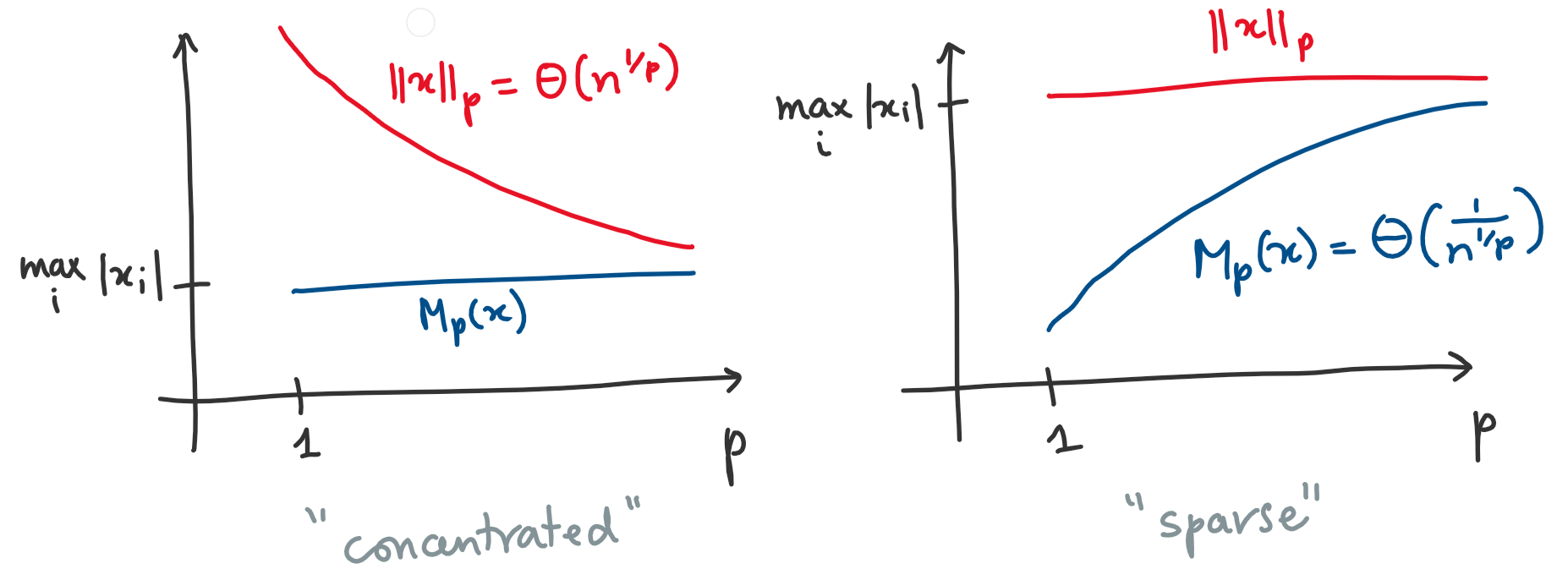
TODO: change “concentrated” to “spread” in this graph #figure
TODO: also make a “table” #figure
Qualities being tracked
We can use ratios between norms to track different qualitative behaviors (the ratios below are $\ge 1$, with $1$ indicating perfection):
- for a vector $x \in \R^n$, the length ratios $\frac{\norm{x}_p}{\norm{x}_q}$ track its sparsity;
- for a sequence $a \in \R_{\ge 0}^n$, the mean ratios $\frac{M_q(a)}{M_p(a)}$ track its spreadness;
- for a random variable $\BX$, the moment ratios $\frac{\norm{\BX}_q}{\norm{\BX}_p}$ track its reasonableness;
- by extension, so do the norm ratios $\frac{\norm{f}_q}{\norm{f}_p}$ for a function $f$ (by considering its value $f(\BX)$ over a random input $\BX$);
- for a discrete random variable $\BX$, the power entropy ratios $\f{H_\alpha[\BX]}{H_\beta[\BX]}$ (for $0 \le \alpha < \beta \le \infty$ ) track its flatness.
TODO: add something about Density functions (are inner products like $\inner{f, f^p}$ the right notion?)
See also