$\require{mathtools}
\newcommand{\nc}{\newcommand}
%
%%% GENERIC MATH %%%
%
% Environments
\newcommand{\al}[1]{\begin{align}#1\end{align}} % need this for \tag{} to work
\renewcommand{\r}{\mathrm} % BAD!! does cursed things with accents :((
\renewcommand{\t}{\textrm}
\newcommand{\either}[1]{\begin{cases}#1\end{cases}}
%
% Delimiters
% (I needed to create my own because the MathJax version of \DeclarePairedDelimiter doesn't have \mathopen{} and that messes up the spacing)
% .. one-part
\newcommand{\p}[1]{\mathopen{}\left( #1 \right)}
\renewcommand{\P}[1]{^{\p{#1}}}
\renewcommand{\b}[1]{\mathopen{}\left[ #1 \right]}
\newcommand{\lopen}[1]{\mathopen{}\left( #1 \right]}
\newcommand{\ropen}[1]{\mathopen{}\left[ #1 \right)}
\newcommand{\set}[1]{\mathopen{}\left\{ #1 \right\}}
\newcommand{\abs}[1]{\mathopen{}\left\lvert #1 \right\rvert}
\newcommand{\floor}[1]{\mathopen{}\left\lfloor #1 \right\rfloor}
\newcommand{\ceil}[1]{\mathopen{}\left\lceil #1 \right\rceil}
\newcommand{\round}[1]{\mathopen{}\left\lfloor #1 \right\rceil}
\newcommand{\inner}[1]{\mathopen{}\left\langle #1 \right\rangle}
\newcommand{\norm}[1]{\mathopen{}\left\lVert #1 \strut \right\rVert}
\newcommand{\frob}[1]{\norm{#1}_\mathrm{F}}
\newcommand{\mix}[1]{\mathopen{}\left\lfloor #1 \right\rceil}
%% .. two-part
\newcommand{\inco}[2]{#1 \mathop{}\middle|\mathop{} #2}
\newcommand{\co}[2]{ {\left.\inco{#1}{#2}\right.}}
\newcommand{\cond}{\co} % deprecated
\newcommand{\pco}[2]{\p{\inco{#1}{#2}}}
\newcommand{\bco}[2]{\b{\inco{#1}{#2}}}
\newcommand{\setco}[2]{\set{\inco{#1}{#2}}}
\newcommand{\at}[2]{ {\left.#1\strut\right|_{#2}}}
\newcommand{\pat}[2]{\p{\at{#1}{#2}}}
\newcommand{\bat}[2]{\b{\at{#1}{#2}}}
\newcommand{\para}[2]{#1\strut \mathop{}\middle\|\mathop{} #2}
\newcommand{\ppa}[2]{\p{\para{#1}{#2}}}
\newcommand{\pff}[2]{\p{\ff{#1}{#2}}}
\newcommand{\bff}[2]{\b{\ff{#1}{#2}}}
\newcommand{\bffco}[4]{\bff{\cond{#1}{#2}}{\cond{#3}{#4}}}
\newcommand{\sm}[1]{\p{\begin{smallmatrix}#1\end{smallmatrix}}}
%
% Greek
\newcommand{\eps}{\epsilon}
\newcommand{\veps}{\varepsilon}
\newcommand{\vpi}{\varpi}
% the following cause issues with real LaTeX tho :/ maybe consider naming it \fhi instead?
\let\fi\phi % because it looks like an f
\let\phi\varphi % because it looks like a p
\renewcommand{\th}{\theta}
\newcommand{\Th}{\Theta}
\newcommand{\om}{\omega}
\newcommand{\Om}{\Omega}
%
% Miscellaneous
\newcommand{\LHS}{\mathrm{LHS}}
\newcommand{\RHS}{\mathrm{RHS}}
\DeclareMathOperator{\cst}{const}
% .. operators
\DeclareMathOperator{\poly}{poly}
\DeclareMathOperator{\polylog}{polylog}
\DeclareMathOperator{\quasipoly}{quasipoly}
\DeclareMathOperator{\negl}{negl}
\DeclareMathOperator*{\argmin}{arg\thinspace min}
\DeclareMathOperator*{\argmax}{arg\thinspace max}
\DeclareMathOperator{\diag}{diag}
% .. functions
\DeclareMathOperator{\id}{id}
\DeclareMathOperator{\sign}{sign}
\DeclareMathOperator{\step}{step}
\DeclareMathOperator{\err}{err}
\DeclareMathOperator{\ReLU}{ReLU}
\DeclareMathOperator{\softmax}{softmax}
% .. analysis
\let\d\undefined
\newcommand{\d}{\operatorname{d}\mathopen{}}
\newcommand{\dd}[1]{\operatorname{d}^{#1}\mathopen{}}
\newcommand{\df}[2]{ {\f{\d #1}{\d #2}}}
\newcommand{\ds}[2]{ {\sl{\d #1}{\d #2}}}
\newcommand{\ddf}[3]{ {\f{\dd{#1} #2}{\p{\d #3}^{#1}}}}
\newcommand{\dds}[3]{ {\sl{\dd{#1} #2}{\p{\d #3}^{#1}}}}
\renewcommand{\part}{\partial}
\newcommand{\ppart}[1]{\part^{#1}}
\newcommand{\partf}[2]{\f{\part #1}{\part #2}}
\newcommand{\parts}[2]{\sl{\part #1}{\part #2}}
\newcommand{\ppartf}[3]{ {\f{\ppart{#1} #2}{\p{\part #3}^{#1}}}}
\newcommand{\pparts}[3]{ {\sl{\ppart{#1} #2}{\p{\part #3}^{#1}}}}
\newcommand{\grad}[1]{\mathop{\nabla\!_{#1}}}
% .. sets
\newcommand{\es}{\emptyset}
\newcommand{\N}{\mathbb{N}}
\newcommand{\Z}{\mathbb{Z}}
\newcommand{\R}{\mathbb{R}}
\newcommand{\Rge}{\R_{\ge 0}}
\newcommand{\Rgt}{\R_{> 0}}
\newcommand{\C}{\mathbb{C}}
\newcommand{\F}{\mathbb{F}}
\newcommand{\zo}{\set{0,1}}
\newcommand{\pmo}{\set{\pm 1}}
\newcommand{\zpmo}{\set{0,\pm 1}}
% .... set operations
\newcommand{\sse}{\subseteq}
\newcommand{\out}{\not\in}
\newcommand{\minus}{\setminus}
\newcommand{\inc}[1]{\union \set{#1}} % "including"
\newcommand{\exc}[1]{\setminus \set{#1}} % "except"
% .. over and under
\renewcommand{\ss}[1]{_{\substack{#1}}}
\newcommand{\OB}{\overbrace}
\newcommand{\ob}[2]{\OB{#1}^\t{#2}}
\newcommand{\UB}{\underbrace}
\newcommand{\ub}[2]{\UB{#1}_\t{#2}}
\newcommand{\ol}{\overline}
\newcommand{\tld}{\widetilde} % deprecated
\renewcommand{\~}{\widetilde}
\newcommand{\HAT}{\widehat} % deprecated
\renewcommand{\^}{\widehat}
\newcommand{\rt}[1]{ {\sqrt{#1}}}
\newcommand{\for}[2]{_{#1=1}^{#2}}
\newcommand{\sfor}{\sum\for}
\newcommand{\pfor}{\prod\for}
% .... two-part
\newcommand{\f}{\frac}
\renewcommand{\sl}[2]{#1 /\mathopen{}#2}
\newcommand{\ff}[2]{\mathchoice{\begin{smallmatrix}\displaystyle\vphantom{\p{#1}}#1\\[-0.05em]\hline\\[-0.05em]\hline\displaystyle\vphantom{\p{#2}}#2\end{smallmatrix}}{\begin{smallmatrix}\vphantom{\p{#1}}#1\\[-0.1em]\hline\\[-0.1em]\hline\vphantom{\p{#2}}#2\end{smallmatrix}}{\begin{smallmatrix}\vphantom{\p{#1}}#1\\[-0.1em]\hline\\[-0.1em]\hline\vphantom{\p{#2}}#2\end{smallmatrix}}{\begin{smallmatrix}\vphantom{\p{#1}}#1\\[-0.1em]\hline\\[-0.1em]\hline\vphantom{\p{#2}}#2\end{smallmatrix}}}
% .. arrows
\newcommand{\from}{\leftarrow}
\DeclareMathOperator*{\<}{\!\;\longleftarrow\;\!}
\let\>\undefined
\DeclareMathOperator*{\>}{\!\;\longrightarrow\;\!}
\let\-\undefined
\DeclareMathOperator*{\-}{\!\;\longleftrightarrow\;\!}
\newcommand{\so}{\implies}
% .. operators and relations
\renewcommand{\*}{\cdot}
\newcommand{\x}{\times}
\newcommand{\ox}{\otimes}
\newcommand{\OX}[1]{^{\ox #1}}
\newcommand{\sr}{\stackrel}
\newcommand{\ce}{\coloneqq}
\newcommand{\ec}{\eqqcolon}
\newcommand{\ap}{\approx}
\newcommand{\ls}{\lesssim}
\newcommand{\gs}{\gtrsim}
% .. punctuation and spacing
\renewcommand{\.}[1]{#1\dots#1}
\newcommand{\ts}{\thinspace}
\newcommand{\q}{\quad}
\newcommand{\qq}{\qquad}
%
%
%%% SPECIALIZED MATH %%%
%
% Logic and bit operations
\newcommand{\fa}{\forall}
\newcommand{\ex}{\exists}
\renewcommand{\and}{\wedge}
\newcommand{\AND}{\bigwedge}
\renewcommand{\or}{\vee}
\newcommand{\OR}{\bigvee}
\newcommand{\xor}{\oplus}
\newcommand{\XOR}{\bigoplus}
\newcommand{\union}{\cup}
\newcommand{\dunion}{\sqcup}
\newcommand{\inter}{\cap}
\newcommand{\UNION}{\bigcup}
\newcommand{\DUNION}{\bigsqcup}
\newcommand{\INTER}{\bigcap}
\newcommand{\comp}{\overline}
\newcommand{\true}{\r{true}}
\newcommand{\false}{\r{false}}
\newcommand{\tf}{\set{\true,\false}}
\DeclareMathOperator{\One}{\mathbb{1}}
\DeclareMathOperator{\1}{\mathbb{1}} % use \mathbbm instead if using real LaTeX
\DeclareMathOperator{\LSB}{LSB}
%
% Linear algebra
\newcommand{\spn}{\mathrm{span}} % do NOT use \span because it causes misery with amsmath
\DeclareMathOperator{\rank}{rank}
\DeclareMathOperator{\proj}{proj}
\DeclareMathOperator{\dom}{dom}
\DeclareMathOperator{\Img}{Im}
\DeclareMathOperator{\tr}{tr}
\DeclareMathOperator{\perm}{perm}
\DeclareMathOperator{\haf}{haf}
\newcommand{\transp}{\mathsf{T}}
\newcommand{\T}{^\transp}
\newcommand{\par}{\parallel}
% .. named tensors
\newcommand{\namedtensorstrut}{\vphantom{fg}} % milder than \mathstrut
\newcommand{\name}[1]{\mathsf{\namedtensorstrut #1}}
\newcommand{\nbin}[2]{\mathbin{\underset{\substack{#1}}{\namedtensorstrut #2}}}
\newcommand{\ndot}[1]{\nbin{#1}{\odot}}
\newcommand{\ncat}[1]{\nbin{#1}{\oplus}}
\newcommand{\nsum}[1]{\sum\limits_{\substack{#1}}}
\newcommand{\nfun}[2]{\mathop{\underset{\substack{#1}}{\namedtensorstrut\mathrm{#2}}}}
\newcommand{\ndef}[2]{\newcommand{#1}{\name{#2}}}
\newcommand{\nt}[1]{^{\transp(#1)}}
%
% Probability
\newcommand{\tri}{\triangle}
\newcommand{\Normal}{\mathcal{N}}
\newcommand{\Exp}{\mathcal{Exp}}
% .. operators
\DeclareMathOperator{\supp}{supp}
\let\Pr\undefined
\DeclareMathOperator*{\Pr}{Pr}
\DeclareMathOperator*{\G}{\mathbb{G}}
\DeclareMathOperator*{\Odds}{Od}
\DeclareMathOperator*{\E}{E}
\DeclareMathOperator*{\Var}{Var}
\DeclareMathOperator*{\Cov}{Cov}
\DeclareMathOperator*{\K}{K}
\DeclareMathOperator*{\corr}{corr}
\DeclareMathOperator*{\median}{median}
\DeclareMathOperator*{\maj}{maj}
% ... information theory
\let\H\undefined
\DeclareMathOperator*{\H}{H}
\DeclareMathOperator*{\I}{I}
\DeclareMathOperator*{\D}{D}
\DeclareMathOperator*{\KL}{KL}
% .. other divergences
\newcommand{\dTV}{d_{\mathrm{TV}}}
\newcommand{\dHel}{d_{\mathrm{Hel}}}
\newcommand{\dJS}{d_{\mathrm{JS}}}
%
% Polynomials
\DeclareMathOperator{\He}{He}
\DeclareMathOperator{\coeff}{coeff}
%
%%% SPECIALIZED COMPUTER SCIENCE %%%
%
% Complexity classes
% .. keywords
\newcommand{\coclass}{\mathsf{co}}
\newcommand{\Prom}{\mathsf{Promise}}
% .. classical
\newcommand{\PTIME}{\mathsf{P}}
\newcommand{\NP}{\mathsf{NP}}
\newcommand{\coNP}{\coclass\NP}
\newcommand{\PH}{\mathsf{PH}}
\newcommand{\PSPACE}{\mathsf{PSPACE}}
\renewcommand{\L}{\mathsf{L}}
\newcommand{\EXP}{\mathsf{EXP}}
\newcommand{\NEXP}{\mathsf{NEXP}}
% .. probabilistic
\newcommand{\formost}{\mathsf{Я}}
\newcommand{\RP}{\mathsf{RP}}
\newcommand{\BPP}{\mathsf{BPP}}
\newcommand{\ZPP}{\mathsf{ZPP}}
\newcommand{\MA}{\mathsf{MA}}
\newcommand{\AM}{\mathsf{AM}}
\newcommand{\IP}{\mathsf{IP}}
\newcommand{\RL}{\mathsf{RL}}
% .. circuits
\newcommand{\NC}{\mathsf{NC}}
\newcommand{\AC}{\mathsf{AC}}
\newcommand{\ACC}{\mathsf{ACC}}
\newcommand{\ThrC}{\mathsf{TC}}
\newcommand{\Ppoly}{\mathsf{P}/\poly}
\newcommand{\Lpoly}{\mathsf{L}/\poly}
% .. resources
\newcommand{\TIME}{\mathsf{TIME}}
\newcommand{\NTIME}{\mathsf{NTIME}}
\newcommand{\SPACE}{\mathsf{SPACE}}
\newcommand{\TISP}{\mathsf{TISP}}
\newcommand{\SIZE}{\mathsf{SIZE}}
% .. custom
\newcommand{\NCP}{\mathsf{NCP}}
%
% Boolean analysis
\newcommand{\harpoon}{\!\upharpoonright\!}
\newcommand{\rr}[2]{#1\harpoon_{#2}}
\newcommand{\Fou}[1]{\widehat{#1}}
\DeclareMathOperator{\Ind}{\mathrm{Ind}}
\DeclareMathOperator{\Inf}{\mathrm{Inf}}
\newcommand{\Der}[1]{\operatorname{D}_{#1}\mathopen{}}
% \newcommand{\Exp}[1]{\operatorname{E}_{#1}\mathopen{}}
\DeclareMathOperator{\Stab}{\mathrm{Stab}}
\DeclareMathOperator{\Tau}{T}
\DeclareMathOperator{\sens}{\mathrm{s}}
\DeclareMathOperator{\bsens}{\mathrm{bs}}
\DeclareMathOperator{\fbsens}{\mathrm{fbs}}
\DeclareMathOperator{\Cert}{\mathrm{C}}
\DeclareMathOperator{\DT}{\mathrm{DT}}
\DeclareMathOperator{\CDT}{\mathrm{CDT}} % canonical
\DeclareMathOperator{\ECDT}{\mathrm{ECDT}}
\DeclareMathOperator{\CDTv}{\mathrm{CDT_{vars}}}
\DeclareMathOperator{\ECDTv}{\mathrm{ECDT_{vars}}}
\DeclareMathOperator{\CDTt}{\mathrm{CDT_{terms}}}
\DeclareMathOperator{\ECDTt}{\mathrm{ECDT_{terms}}}
\DeclareMathOperator{\CDTw}{\mathrm{CDT_{weighted}}}
\DeclareMathOperator{\ECDTw}{\mathrm{ECDT_{weighted}}}
\DeclareMathOperator{\AvgDT}{\mathrm{AvgDT}}
\DeclareMathOperator{\PDT}{\mathrm{PDT}} % partial decision tree
\DeclareMathOperator{\DTsize}{\mathrm{DT_{size}}}
\DeclareMathOperator{\W}{\mathbf{W}}
% .. functions (small caps sadly doesn't work)
\DeclareMathOperator{\Par}{\mathrm{Par}}
\DeclareMathOperator{\Maj}{\mathrm{Maj}}
\DeclareMathOperator{\HW}{\mathrm{HW}}
\DeclareMathOperator{\Thr}{\mathrm{Thr}}
\DeclareMathOperator{\Tribes}{\mathrm{Tribes}}
\DeclareMathOperator{\RotTribes}{\mathrm{RotTribes}}
\DeclareMathOperator{\CycleRun}{\mathrm{CycleRun}}
\DeclareMathOperator{\SAT}{\mathrm{SAT}}
\DeclareMathOperator{\UniqueSAT}{\mathrm{UniqueSAT}}
%
% Dynamic optimality
\newcommand{\OPT}{\mathsf{OPT}}
\newcommand{\Alt}{\mathsf{Alt}}
\newcommand{\Funnel}{\mathsf{Funnel}}
%
% Alignment
\DeclareMathOperator{\Amp}{\mathrm{Amp}}
%
%%% TYPESETTING %%%
%
% In "text"
\newcommand{\heart}{\heartsuit}
\newcommand{\nth}{^\t{th}}
\newcommand{\degree}{^\circ}
\newcommand{\qu}[1]{\text{``}#1\text{''}}
% remove these last two if using real LaTeX
\newcommand{\qed}{\blacksquare}
\newcommand{\qedhere}{\tag*{$\blacksquare$}}
%
% Fonts
% .. bold
\newcommand{\BA}{\boldsymbol{A}}
\newcommand{\BB}{\boldsymbol{B}}
\newcommand{\BC}{\boldsymbol{C}}
\newcommand{\BD}{\boldsymbol{D}}
\newcommand{\BE}{\boldsymbol{E}}
\newcommand{\BF}{\boldsymbol{F}}
\newcommand{\BG}{\boldsymbol{G}}
\newcommand{\BH}{\boldsymbol{H}}
\newcommand{\BI}{\boldsymbol{I}}
\newcommand{\BJ}{\boldsymbol{J}}
\newcommand{\BK}{\boldsymbol{K}}
\newcommand{\BL}{\boldsymbol{L}}
\newcommand{\BM}{\boldsymbol{M}}
\newcommand{\BN}{\boldsymbol{N}}
\newcommand{\BO}{\boldsymbol{O}}
\newcommand{\BP}{\boldsymbol{P}}
\newcommand{\BQ}{\boldsymbol{Q}}
\newcommand{\BR}{\boldsymbol{R}}
\newcommand{\BS}{\boldsymbol{S}}
\newcommand{\BT}{\boldsymbol{T}}
\newcommand{\BU}{\boldsymbol{U}}
\newcommand{\BV}{\boldsymbol{V}}
\newcommand{\BW}{\boldsymbol{W}}
\newcommand{\BX}{\boldsymbol{X}}
\newcommand{\BY}{\boldsymbol{Y}}
\newcommand{\BZ}{\boldsymbol{Z}}
\newcommand{\Ba}{\boldsymbol{a}}
\newcommand{\Bb}{\boldsymbol{b}}
\newcommand{\Bc}{\boldsymbol{c}}
\newcommand{\Bd}{\boldsymbol{d}}
\newcommand{\Be}{\boldsymbol{e}}
\newcommand{\Bf}{\boldsymbol{f}}
\newcommand{\Bg}{\boldsymbol{g}}
\newcommand{\Bh}{\boldsymbol{h}}
\newcommand{\Bi}{\boldsymbol{i}}
\newcommand{\Bj}{\boldsymbol{j}}
\newcommand{\Bk}{\boldsymbol{k}}
\newcommand{\Bl}{\boldsymbol{l}}
\newcommand{\Bm}{\boldsymbol{m}}
\newcommand{\Bn}{\boldsymbol{n}}
\newcommand{\Bo}{\boldsymbol{o}}
\newcommand{\Bp}{\boldsymbol{p}}
\newcommand{\Bq}{\boldsymbol{q}}
\newcommand{\Br}{\boldsymbol{r}}
\newcommand{\Bs}{\boldsymbol{s}}
\newcommand{\Bt}{\boldsymbol{t}}
\newcommand{\Bu}{\boldsymbol{u}}
\newcommand{\Bv}{\boldsymbol{v}}
\newcommand{\Bw}{\boldsymbol{w}}
\newcommand{\Bx}{\boldsymbol{x}}
\newcommand{\By}{\boldsymbol{y}}
\newcommand{\Bz}{\boldsymbol{z}}
\newcommand{\Balpha}{\boldsymbol{\alpha}}
\newcommand{\Bbeta}{\boldsymbol{\beta}}
\newcommand{\Bgamma}{\boldsymbol{\gamma}}
\newcommand{\Bdelta}{\boldsymbol{\delta}}
\newcommand{\Beps}{\boldsymbol{\eps}}
\newcommand{\Bveps}{\boldsymbol{\veps}}
\newcommand{\Bzeta}{\boldsymbol{\zeta}}
\newcommand{\Beta}{\boldsymbol{\eta}}
\newcommand{\Btheta}{\boldsymbol{\theta}}
\newcommand{\Bth}{\boldsymbol{\th}}
\newcommand{\Biota}{\boldsymbol{\iota}}
\newcommand{\Bkappa}{\boldsymbol{\kappa}}
\newcommand{\Blambda}{\boldsymbol{\lambda}}
\newcommand{\Bmu}{\boldsymbol{\mu}}
\newcommand{\Bnu}{\boldsymbol{\nu}}
\newcommand{\Bxi}{\boldsymbol{\xi}}
\newcommand{\Bpi}{\boldsymbol{\pi}}
\newcommand{\Bvpi}{\boldsymbol{\vpi}}
\newcommand{\Brho}{\boldsymbol{\rho}}
\newcommand{\Bsigma}{\boldsymbol{\sigma}}
\newcommand{\Btau}{\boldsymbol{\tau}}
\newcommand{\Bupsilon}{\boldsymbol{\upsilon}}
\newcommand{\Bphi}{\boldsymbol{\phi}}
\newcommand{\Bfi}{\boldsymbol{\fi}}
\newcommand{\Bchi}{\boldsymbol{\chi}}
\newcommand{\Bpsi}{\boldsymbol{\psi}}
\newcommand{\Bom}{\boldsymbol{\om}}
% .. calligraphic
\newcommand{\CA}{\mathcal{A}}
\newcommand{\CB}{\mathcal{B}}
\newcommand{\CC}{\mathcal{C}}
\newcommand{\CD}{\mathcal{D}}
\newcommand{\CE}{\mathcal{E}}
\newcommand{\CF}{\mathcal{F}}
\newcommand{\CG}{\mathcal{G}}
\newcommand{\CH}{\mathcal{H}}
\newcommand{\CI}{\mathcal{I}}
\newcommand{\CJ}{\mathcal{J}}
\newcommand{\CK}{\mathcal{K}}
\newcommand{\CL}{\mathcal{L}}
\newcommand{\CM}{\mathcal{M}}
\newcommand{\CN}{\mathcal{N}}
\newcommand{\CO}{\mathcal{O}}
\newcommand{\CP}{\mathcal{P}}
\newcommand{\CQ}{\mathcal{Q}}
\newcommand{\CR}{\mathcal{R}}
\newcommand{\CS}{\mathcal{S}}
\newcommand{\CT}{\mathcal{T}}
\newcommand{\CU}{\mathcal{U}}
\newcommand{\CV}{\mathcal{V}}
\newcommand{\CW}{\mathcal{W}}
\newcommand{\CX}{\mathcal{X}}
\newcommand{\CY}{\mathcal{Y}}
\newcommand{\CZ}{\mathcal{Z}}
% .. typewriter
\newcommand{\TA}{\mathtt{A}}
\newcommand{\TB}{\mathtt{B}}
\newcommand{\TC}{\mathtt{C}}
\newcommand{\TD}{\mathtt{D}}
\newcommand{\TE}{\mathtt{E}}
\newcommand{\TF}{\mathtt{F}}
\newcommand{\TG}{\mathtt{G}}
\renewcommand{\TH}{\mathtt{H}}
\newcommand{\TI}{\mathtt{I}}
\newcommand{\TJ}{\mathtt{J}}
\newcommand{\TK}{\mathtt{K}}
\newcommand{\TL}{\mathtt{L}}
\newcommand{\TM}{\mathtt{M}}
\newcommand{\TN}{\mathtt{N}}
\newcommand{\TO}{\mathtt{O}}
\newcommand{\TP}{\mathtt{P}}
\newcommand{\TQ}{\mathtt{Q}}
\newcommand{\TR}{\mathtt{R}}
\newcommand{\TS}{\mathtt{S}}
\newcommand{\TT}{\mathtt{T}}
\newcommand{\TU}{\mathtt{U}}
\newcommand{\TV}{\mathtt{V}}
\newcommand{\TW}{\mathtt{W}}
\newcommand{\TX}{\mathtt{X}}
\newcommand{\TY}{\mathtt{Y}}
\newcommand{\TZ}{\mathtt{Z}}
%
% LEVELS OF CLOSENESS (basically deprecated)
\newcommand{\scirc}[1]{\sr{\circ}{#1}}
\newcommand{\sdot}[1]{\sr{.}{#1}}
\newcommand{\slog}[1]{\sr{\log}{#1}}
\newcommand{\createClosenessLevels}[7]{
\newcommand{#2}{\mathrel{(#1)}}
\newcommand{#3}{\mathrel{#1}}
\newcommand{#4}{\mathrel{#1\!\!#1}}
\newcommand{#5}{\mathrel{#1\!\!#1\!\!#1}}
\newcommand{#6}{\mathrel{(\sdot{#1})}}
\newcommand{#7}{\mathrel{(\slog{#1})}}
}
\let\lt\undefined
\let\gt\undefined
% .. vanilla versions (is it within a constant?)
\newcommand{\ez}{\scirc=}
\newcommand{\eq}{\simeq}
\newcommand{\eqq}{\mathrel{\eq\!\!\eq}}
\newcommand{\eqqq}{\mathrel{\eq\!\!\eq\!\!\eq}}
\newcommand{\lez}{\scirc\le}
\renewcommand{\lq}{\preceq}
\newcommand{\lqq}{\mathrel{\lq\!\!\lq}}
\newcommand{\lqqq}{\mathrel{\lq\!\!\lq\!\!\lq}}
\newcommand{\gez}{\scirc\ge}
\newcommand{\gq}{\succeq}
\newcommand{\gqq}{\mathrel{\gq\!\!\gq}}
\newcommand{\gqqq}{\mathrel{\gq\!\!\gq\!\!\gq}}
\newcommand{\lz}{\scirc<}
\newcommand{\lt}{\prec}
\newcommand{\ltt}{\mathrel{\lt\!\!\lt}}
\newcommand{\lttt}{\mathrel{\lt\!\!\lt\!\!\lt}}
\newcommand{\gz}{\scirc>}
\newcommand{\gt}{\succ}
\newcommand{\gtt}{\mathrel{\gt\!\!\gt}}
\newcommand{\gttt}{\mathrel{\gt\!\!\gt\!\!\gt}}
% .. dotted versions (is it equal in the limit?)
\newcommand{\ed}{\sdot=}
\newcommand{\eqd}{\sdot\eq}
\newcommand{\eqqd}{\sdot\eqq}
\newcommand{\eqqqd}{\sdot\eqqq}
\newcommand{\led}{\sdot\le}
\newcommand{\lqd}{\sdot\lq}
\newcommand{\lqqd}{\sdot\lqq}
\newcommand{\lqqqd}{\sdot\lqqq}
\newcommand{\ged}{\sdot\ge}
\newcommand{\gqd}{\sdot\gq}
\newcommand{\gqqd}{\sdot\gqq}
\newcommand{\gqqqd}{\sdot\gqqq}
\newcommand{\ld}{\sdot<}
\newcommand{\ltd}{\sdot\lt}
\newcommand{\lttd}{\sdot\ltt}
\newcommand{\ltttd}{\sdot\lttt}
\newcommand{\gd}{\sdot>}
\newcommand{\gtd}{\sdot\gt}
\newcommand{\gttd}{\sdot\gtt}
\newcommand{\gtttd}{\sdot\gttt}
% .. log versions (is it equal up to log?)
\newcommand{\elog}{\slog=}
\newcommand{\eqlog}{\slog\eq}
\newcommand{\eqqlog}{\slog\eqq}
\newcommand{\eqqqlog}{\slog\eqqq}
\newcommand{\lelog}{\slog\le}
\newcommand{\lqlog}{\slog\lq}
\newcommand{\lqqlog}{\slog\lqq}
\newcommand{\lqqqlog}{\slog\lqqq}
\newcommand{\gelog}{\slog\ge}
\newcommand{\gqlog}{\slog\gq}
\newcommand{\gqqlog}{\slog\gqq}
\newcommand{\gqqqlog}{\slog\gqqq}
\newcommand{\llog}{\slog<}
\newcommand{\ltlog}{\slog\lt}
\newcommand{\lttlog}{\slog\ltt}
\newcommand{\ltttlog}{\slog\lttt}
\newcommand{\glog}{\slog>}
\newcommand{\gtlog}{\slog\gt}
\newcommand{\gttlog}{\slog\gtt}
\newcommand{\gtttlog}{\slog\gttt}$
The information divergence measures the information gained when going from a prior distribution $P$ to a posterior distribution $Q$, i.e. how much you learned if you believed something was distributed according to $P$ and now believe it is distribution $Q$ based on evidence. Concretely, it measures (the logarithm of) how much more “confident” you now are about your current beliefs:
\[
\D\pff{Q}{P} \ce \E_{x \sim Q}\b{\log\frac{Q(x)}{P(x)}}.
\]
We can extend the notion to random variables:
\[
\D\bff{\BX'}{\BX} \ce \E_{\Bx \sim \b{\BX'}}\b{\log\frac{\Pr[\BX'=\Bx]}{\Pr[\BX=\Bx]}}
\]
(note that this is only a function of the distributions of $\BX$ and $\BX'$ seen separately; we’re not thinking of them as jointly distributed).
Interpretations
The information divergence can be understood in three main ways, as a measure of
- the information gained when updating from $P$ to $Q$,
- the specificity of draws from $Q$ compared to $P$,
- and the unlikelihood of $P$ as a model given that your observations suggest $Q$.
And all of these links ultimately rely on the fact that the information divergence adds up nicely if we compare several independent samples from both $P$ and $Q$. A good intuition is that as $n$ grows, $Q^n$ looks more and more like we just conditioned $P^n$ on some event of probability $\exp\p{-n \D\pff{Q}{P}}$.
See Six (and a half) intuitions for KL divergence for more intuitions, in particular ones related to betting.
The information divergence is the core of information theory because it defines what it means to gain information based on observations. In particular,
- the mutual information $\I[\BX;\BY]$ is the average information we gain about $\BY$ when observing $\BX$ (and vice versa): $\I[\BX;\BY] = \E\b{\D\bff{\cond{\BY}{\BX}}{\BY}} = \E\b{\D\bff{\cond{\BX}{\BY}}{\BX}}$;
- and the entropy $\H[\BX]$ is the average information we gain about $\BX$ when observing it: $\H[\BX] = \I[\BX;\BX] = \E\b{\D\bff{\cond{\BX}{\BX}}{\BX}} = \E\b{\log \f 1 {[\BX](\BX)}}$.
Specificity of draws from $Q$
The prior $P$ should be thought of as a more uniform baseline, and the posterior $Q$ as taking more specific or weird values, and being the interesting object of study. In particular, the definition only makes sense if the support of $Q$ is contained in the support of $P$.
Asymptotic likelihood ratio
The information divergence $\D\pff{Q}{P}$ quantifies the typical likelihood ratio between $Q$ and $P$ for large samples of independent draws from $Q$. More precisely, for any fixed tolerance $\delta>0$, if you draw a sample $\BS \sim Q^n$, then we have
\[
\log \f{Q^n(\BS)}{P^n(\BS)} \in n\p{\D\pff{Q}{P} \pm o(1)}
\]
except with probability $\delta$.
In particular, this means that the information divergence measures the amount of selection pressure you typically need to pick out a sample that roughly looks like it came from $Q$ from $n$-samples that actually came from $P$ (here, “roughly” means we might give up on reproducing a $\delta$ part of the distribution of $Q^n$). If you want to match the distribution exactly, this is measured by max-divergence instead, no matter what $n$ is.
Entropy deficit
If $P$ is uniform over some sample space $\CX$, then $\D\pff{Q}{P}$ measures the difference between the entropies $\H(P)-\H(Q)$. Since uniform distributions maximize entropy, this represents how much entropy $Q$ is potentially “missing out” on, i.e. its entropy deficit.
Evidence against $P$
$\D\pff{Q}{P}$ is the “amount of evidence against $P$” that you get per sample: it’s the amortized log-unlikelihood that a large sample from $P$ ends up empirically distributed in a way that looks roughly like $Q$. Indeed, suppose $P,Q$ are distributions over $[m]$ (and denoting $p_i \ce P(i)$ and $q_i \ce Q(i)$), then the probability that we draw $n$ samples from $P$ and each $i \in [m]$ appears $\ap q_in$ times is roughly
\[
\al{
\binom{n}{\ap q_1n, \dotsc, \approx q_mn} \prod p_i^{q_i n}
&= \UB{\binom{n}{\ap q_1n, \dotsc, \approx q_mn} \prod q_i^{q_i n}}_\text{probability that a sample from $Q$ ends up looking roughly like $Q$}
\prod\p{\f{p_i}{q_i}}^{q_in}\\
&\approx \prod\p{\f{p_i}{q_i}}^{q_in}\\
&= \exp\p{-\D\pff{Q}{P}n}.
}
\]
Hypothesis testing
As a consequence, there exists a test for “detecting” based on a large enough number of samples, such that
- if the samples are from $Q$, the test comes up positive with high probability in $n$ (the test is sensitive),
- and if the samples are from $P$, the test comes up positive with probability at most $2^{-n\p{\D\pff{Q}{P}-o(1)}}$ (the test is extremely specific).
So if the test comes up positive, the belief that the samples came from $P$ as opposed to $Q$ becomes extremely untenable as $n$ grows.
Learning theory: minimizing divergence maximizes likelihood of $P$
In learning theory, we can let $Q$ be the target real-world distribution, and $P$ be the distribution represented by a simplified generative model from a restricted class. Then, minimizing $\D\pff{Q}{P}$ corresponds to picking the model $P$ that minimizes the information we still have to learn per sample. Since $Q$ is fixed, this is equivalent to minimizing the cross-entropy $\H\pff{Q}{P}$. #to-write actually that’s an interpretation for the cross entropy not the information div
In terms of dynamics, the model knows less than nature, so it starts out more uncertain, and therefore $P$ is generally more uniform, and gives fairly low probabilities to everything. Minimizing the information divergence $\D\pff{Q}{P}$ will incentivize $P$ to give higher probabilities to values that are frequent in $Q$.
If instead we define $Q$ to be uniform over the training data, then the $P$ that minimizes $\D\pff{Q}{P}$ is the maximum likelihood model.
#to-write explicitly model Q as P conditioned on E?
Properties
Nonnegativity
As a ratio divergence, it is always nonnegative, and is $0$ iff $P$ and $Q$ are identical.
Asymptotics
Using its nonnegative form, we get
\[
\D\pff{Q}{P}
= \Theta\p{\sum_x
\begin{cases}
P(x)\p{\f{Q(x)}{P(x)}-1}^2 & \text{if $\f{Q(x)}{P(x)} \le O(1)$}\\
Q(x)\log \frac{Q(x)}{P(x)} & \text{otherwise}
\end{cases}
}
\]
(change $\sum_x$ to $\int_x$ if $P,Q$ are continuous probability distributions).
Additivity
Independent priors and posteriors
If the priors and posteriors are both product distributions, then the divergence can be decomposed:
\[
\al{
\D\pff{Q_1 \dotsm Q_n}{P_1 \dotsm P_n}
&= \E_{\Bx \sim Q_1 \dotsm Q_n}\b{\log\frac{Q_1(\Bx_1) \dotsm Q_n(\Bx_n)}{P_1(\Bx_1) \dotsm P_n(\Bx_n)}}\\
&= \E_{\Bx \sim Q_1 \dotsm Q_n}\b{\log\frac{Q_1(\Bx_1)}{P_1(\Bx_1)} + \dotsb + \log\f{Q_n(\Bx_n)}{P_n(\Bx_n)}}\\
&= \D\pff{Q_1}{P_1} + \dotsb + \D\pff{Q_n}{P_n}.
}
\]
This situation mostly occurs when we believe these $n$ values $\Bx_1, \ldots, \Bx_n$ are independent samples from an identical random process, and we want to update our belief about the random process but not about the values themselves. When that’s the case, the additivity simplifies to
\[
\D\pff{Q^n}{P^n} = n\D\pff{Q}{P}.
\]
Independent priors
If the prior variables $\BX$ and $\BY$ are independent, then we have superadditivity (this generalizes the superadditivity of entropy deficit):
\[
\D\bff{\BX',\BY'}{\BX,\BY} \geq \D\bff{\BX'}{\BX}+\D\bff{\BY'}{\BY}.
\]
Intuitively, this is because you can notice more ways in which $\BX',\BY'$ differ from $\BX,\BY$ if you get to look at the together and cross-check. Formally, we have
\[
\al{
&\D\bff{\BX',\BY'}{\BX,\BY} - \D\bff{\BX'}{\BX}-\D\bff{\BY'}{\BY}\\
&\qquad= \E_{(x,y) \sim (\BX',\BY')}\b{\frac{\Pr[\BX'=x\and\BY'=y]\Pr[\BX=x]\Pr[\BY=y]}{\Pr[\BX=x\and\BY=y]\Pr[\BX'=x]\Pr[\BY'=y]}}\\
&\qquad= \E_{(x,y) \sim (\BX',\BY')}\b{\frac{\Pr[\BX'=x\and\BY'=y]}{\Pr[\BX'=x]\Pr[\BY'=y]}}\\
&\qquad= \I\b{\BX';\BY'}\\
&\qquad\ge 0.
}
\]
I’m not sure about the case when $\BX'$ and $\BY'$ are independent, but it seems less natural anyway: why would the posterior be independent if the prior isn’t?
#to-write
- also rewrite in distribution form?
- no actually maybe it’s better to write it like $\D\bff{\at{(\BX,\BY)}{\BE}}{\BX,\BY}$?
- ohh hold on this is where “total correlation” comes in right?
- can you also write that one as a sum of mutual information? or of interaction informations?
- is it the sum of all the interaction informations
-
| is I[X1,X2] + I[X3;X2 |
X1] + I[X4;X3 |
X1,X2] etc? |
- ==okay this is highly relevant to my plight with the small-read local lemma!==
- also explain typical situation: were from a common process but now have observed something about the values in aggregate
- link to the information theoretic proof of the Chernoff bound
General case
In general, though, the quantities $\D\bff{\BX',\BY'}{\BX,\BY}$ and $\D\bff{\BX'}{\BX}+\D\bff{\BY'}{\BY}$ are not comparable: information divergence is neither subadditive nor superadditive. For example, even when $\BX$ and $\BY$ are independent, we can have
\[
\left\{
\al{
&\D\bff{\BX'}{\BX} = \D\bff{\BX'}{\BX} = 0\\
&\D\bff{\BX',\BY'}{\BX,\BY} > 0.
}
\right.
\]
On the other hand, by the section on conditional divergence below, we know that $\D\bff{\BX'}{\BX}, \D\bff{\BY'}{\BY} \le \D\bff{\BX',\BY'}{\BX,\BY}$, so
\[
\D\bff{\BX'}{\BX} + \D\bff{\BY'}{\BY} \le 2\D\bff{\BX',\BY'}{\BX,\BY},
\]
and the second example below approximately saturates this bound.
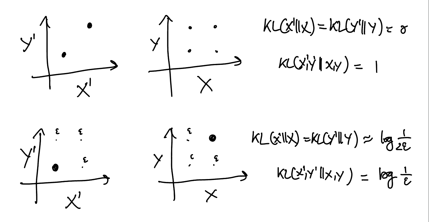
#figure redo the figure with the new notation
Triangle inequality
Sadly, the information divergence doesn’t satisfy the triangle inequality. In general, $\D\pff{Q}{P} + \D\pff{R}{Q}$ can be much smaller than $\D\pff{R}{P}$. In fact, we can make $\D\pff R P$ while keeping $\D\pff{Q}{P} + \D\pff{R}{Q}$ arbitrarily small by arbitrarily large by zooming into a value from $P$ to $Q$ and again from $Q$ to $R$ while taking care to keep it just small enough that it doesn’t get noticed in $\D\pff{Q}{P}$ or $\D\pff{R}{Q}$.
Some representative examples:
- “zoom regime”:
- example 1
- if the distributions are
- $P$ uniform over $[D]$
- $Q$ gives $\f{1}{\log D}$ probability to the value $1$ and is otherwise uniform
- $R$ is $1$ deterministically
- then
- $\D\pff{Q}{P} \le \f{1}{\log D} \log \p{\f{D}{\log D}} \le 1$
- $\D\pff{R}{Q} = \log \log D$
- $\D\pff{R}{P} = \log D$
- example 2 (even worse)
- if the distributions are
- $P \ce \CB\p{\f1{\exp\exp\D}}$
- $Q \ce \CB\p{\f1{\exp D}}$
- $R \ce \CB\p{\f1D}$
- then
- $\D\pff{Q}{P}$ and $\D\pff{R}{Q}$ are both $\le 1$
- but $\D\pff{Q}{P} \ge \exp\Om\p{\D}$
- “tweak regime”:
- if $P \ce B\p{\f12}$, $Q \ce B\p{\f{1+\eps}{2}}$, $R \ce B\p{\f{1+2\eps}{2}}$
- then
- $\D\pff{Q}{P} \sim \D\pff{R}{Q} \sim \f{\eps^2}{2}$
- $\D\pff{R}{P} \sim 2\eps^2$
#to-think I think in general, for any distributions $P$ and $R$, there is a distribution $Q$ such that
\[
\D\pff{Q}{P} + \D\pff{R}{Q} \le (1-\Omega(1))\D\pff{R}{P}.
\]
Minimization
Minimizing $\D\pff{Q}{P}$ over $Q$ is called information projection or mode seeking. We can rewrite it as
\[
\min_Q \UB{\E_{\Bx \sim Q}\b{\log \f1{P(\Bx)}}}_\text{try to hit frequent values under $P$} - \UB{\H(Q)}_\text{try to be broad}.
\]
That is, $Q$ has to trade-off between hitting the most frequent values of $\Bx$ under $P$ and still being as broad as possible. If $Q$ is unconstrained, then the optimum is $Q=P$.
More generally,
- the expression $\log \f1{P(x)}$ doesn’t have to correspond to an actual distribution: we can let it be any energy function $E(x)$
- and we can weight the entropy maximization term by an “temperature” $T$,
in which case the problem becomes
\[
\min_Q \UB{\E_{\Bx \sim Q}\b{E(\Bx)}}_\text{try to hit low energy values} - \UB{T\H(Q)}_\text{try to be broad}.
\]
That is, $Q$ tries to hit the values with the lowest energy, but the higher the temperature $T$ is, the more important the entropy will be, and thus the more uncertain $Q$ will remain. This expression is sometimes called the Helmholtz free energy, and the optimum is given by the Boltzmann distribution $Q(x) \propto \exp\p{-\f{E(x)}T}$, since that’s precisely the distribution $P$ that would have given this minimization problem (up to constants).
#to-write
- link to Variational representations#Information divergence
- generalize this optimization pattern (keeps popping up and almost magical, see
lee--entropy-opt-1.pdf how magical it is that the density takes a simple form, completely unaffected by actual values)
Moment projection: minimizing over $P$
Minimizing $\D\pff{Q}{P}$ over $P$ is called moment projection or mode covering. Since $\D\pff{Q}{P} = \H\pff{Q}{P} - \H(Q)$ and $Q$ is fixed, this is equivalent to minimizing the cross-entropy $\H\pff{Q}{P}$. See Cross-entropy#Minimization.
Special cases
Binary divergence
Let
\[
D\pff{q}{p} \ce q\log\frac{q}{p} + (1-q)\log\frac{1-q}{1-p}
\]
be the divergence between two Bernoullis $B(q)$ and $B(p)$.
Just like the general case, $D\pff{q}{p}$ is nonnegative with $D\pff{q}{p} =0$ iff $q=p$, and strictly convex over $[0,1]^2$. More precisely,
\[
\frac{d^2}{dq^2}D\pff{q}{p} = \frac{1}{q(1-q)}.
\]
Assuming wlog that $p\le 1/2$, the asymptotics are
\[
D\pff{q}{p}
=
\begin{cases}
\Theta\p{p\p{\f{q}{p}-1}^2} & \text{if $0 \le q \le 2p$}\\
\Theta\p{q\log \frac{q}{p}} & \text{if $q \ge 2p$,}
\end{cases}
\]
(where the asymptotic constant is $\f12$ when $q \to p$). In particular, if $p=\f12$ (unbiased) and $q = \f{1+\rho}{2}$ (bias $\rho$), we have $D\pff{q}{p} = \Theta\p{\rho^2}$.
#figure
#to-write
- expected score for logarithmic scoring rule
- full second derivative matrix
- $\D\pff{q}{p} \ge 2(q-p)^2$ (I believe? yup seems right since the second derivative is $\ge 4$)
Normals
#to-write
Conditional divergence
Similar to entropy (but unlike most ratio divergences), we can define the conditional information divergence by taking an average of the divergences of the conditional distributions:
\[
\al{
\D\bffco{\BY'}{\BX'}{\BY}{\BX}
\ce&\ \E_{x \sim \BX'}\b{\D\bff{\at{\BY'}{\BX' = x}}{\at{\BY}{\BX=x}}}\\
=&\ \E_{(x,y) \sim (\BX',\BY')}\b{\log\frac{\Pr[\BY'=y \mid \BX'=x]}{\Pr[\BY=y \mid \BX = x]}},
}
\]
where $\at{\BY}{\BX=x}$ denotes the random variable obtained by conditioning $\BY$ on $\BX=x$.
Chain rule
Similar to conditional entropy, this gives a chain rule:
\[
\al{
\D\bff{\BX',\BY'}{\BX,\BY}
&= \E_{(x,y) \sim (\BX',\BY')}\b{\log\frac{\Pr[\BX' = x \and \BY'=y]}{\Pr[\BX = x \and \BY=y]}}\\
&= \E_{(x,y) \sim (\BX',\BY')}\b{\log\frac{\Pr[\BX' = x]\Pr[\BY'=y\mid \BX'=x]}{\Pr[\BX = x] \Pr[\BY=y \mid \BX=x]}}\\
&= \D\bff{\BX'}{\BX} + \D\bffco{\BY'}{\BX'}{\BY}{\BX},
}
\]
which immediately shows that adding data can only increase the divergence.
Mixtures and convexity
Since information divergence is neither subadditive nor superadditive, $\D\bffco{\BY'}{\BX'}{\BY}{\BX}$ is sometimes bigger and sometimes smaller than $\D\bff{\BY'}{\BY}$. However, like any ratio divergence when $\BX$ and $\BX'$ are the same variable, we have
\[
\D\bff{\BY'}{\BY} \le \D\bff{\BX,\BY'}{\BX,\BY} = \D\bffco{\BY'}{\BX}{\BY}{\BX}.
\]
That is, conditioning by the same variable can only increase the divergence, which is equivalent to saying that the information divergence is convex.
See also