$\require{mathtools}
\newcommand{\nc}{\newcommand}
%
%%% GENERIC MATH %%%
%
% Environments
\newcommand{\al}[1]{\begin{align}#1\end{align}} % need this for \tag{} to work
\renewcommand{\r}{\mathrm} % BAD!! does cursed things with accents :((
\renewcommand{\t}{\textrm}
\newcommand{\either}[1]{\begin{cases}#1\end{cases}}
%
% Delimiters
% (I needed to create my own because the MathJax version of \DeclarePairedDelimiter doesn't have \mathopen{} and that messes up the spacing)
% .. one-part
\newcommand{\p}[1]{\mathopen{}\left( #1 \right)}
\renewcommand{\P}[1]{^{\p{#1}}}
\renewcommand{\b}[1]{\mathopen{}\left[ #1 \right]}
\newcommand{\lopen}[1]{\mathopen{}\left( #1 \right]}
\newcommand{\ropen}[1]{\mathopen{}\left[ #1 \right)}
\newcommand{\set}[1]{\mathopen{}\left\{ #1 \right\}}
\newcommand{\abs}[1]{\mathopen{}\left\lvert #1 \right\rvert}
\newcommand{\floor}[1]{\mathopen{}\left\lfloor #1 \right\rfloor}
\newcommand{\ceil}[1]{\mathopen{}\left\lceil #1 \right\rceil}
\newcommand{\round}[1]{\mathopen{}\left\lfloor #1 \right\rceil}
\newcommand{\inner}[1]{\mathopen{}\left\langle #1 \right\rangle}
\newcommand{\norm}[1]{\mathopen{}\left\lVert #1 \strut \right\rVert}
\newcommand{\frob}[1]{\norm{#1}_\mathrm{F}}
\newcommand{\mix}[1]{\mathopen{}\left\lfloor #1 \right\rceil}
%% .. two-part
\newcommand{\inco}[2]{#1 \mathop{}\middle|\mathop{} #2}
\newcommand{\co}[2]{ {\left.\inco{#1}{#2}\right.}}
\newcommand{\cond}{\co} % deprecated
\newcommand{\pco}[2]{\p{\inco{#1}{#2}}}
\newcommand{\bco}[2]{\b{\inco{#1}{#2}}}
\newcommand{\setco}[2]{\set{\inco{#1}{#2}}}
\newcommand{\at}[2]{ {\left.#1\strut\right|_{#2}}}
\newcommand{\pat}[2]{\p{\at{#1}{#2}}}
\newcommand{\bat}[2]{\b{\at{#1}{#2}}}
\newcommand{\para}[2]{#1\strut \mathop{}\middle\|\mathop{} #2}
\newcommand{\ppa}[2]{\p{\para{#1}{#2}}}
\newcommand{\pff}[2]{\p{\ff{#1}{#2}}}
\newcommand{\bff}[2]{\b{\ff{#1}{#2}}}
\newcommand{\bffco}[4]{\bff{\cond{#1}{#2}}{\cond{#3}{#4}}}
\newcommand{\sm}[1]{\p{\begin{smallmatrix}#1\end{smallmatrix}}}
%
% Greek
\newcommand{\eps}{\epsilon}
\newcommand{\veps}{\varepsilon}
\newcommand{\vpi}{\varpi}
% the following cause issues with real LaTeX tho :/ maybe consider naming it \fhi instead?
\let\fi\phi % because it looks like an f
\let\phi\varphi % because it looks like a p
\renewcommand{\th}{\theta}
\newcommand{\Th}{\Theta}
\newcommand{\om}{\omega}
\newcommand{\Om}{\Omega}
%
% Miscellaneous
\newcommand{\LHS}{\mathrm{LHS}}
\newcommand{\RHS}{\mathrm{RHS}}
\DeclareMathOperator{\cst}{const}
% .. operators
\DeclareMathOperator{\poly}{poly}
\DeclareMathOperator{\polylog}{polylog}
\DeclareMathOperator{\quasipoly}{quasipoly}
\DeclareMathOperator{\negl}{negl}
\DeclareMathOperator*{\argmin}{arg\thinspace min}
\DeclareMathOperator*{\argmax}{arg\thinspace max}
\DeclareMathOperator{\diag}{diag}
% .. functions
\DeclareMathOperator{\id}{id}
\DeclareMathOperator{\sign}{sign}
\DeclareMathOperator{\step}{step}
\DeclareMathOperator{\err}{err}
\DeclareMathOperator{\ReLU}{ReLU}
\DeclareMathOperator{\softmax}{softmax}
% .. analysis
\let\d\undefined
\newcommand{\d}{\operatorname{d}\mathopen{}}
\newcommand{\dd}[1]{\operatorname{d}^{#1}\mathopen{}}
\newcommand{\df}[2]{ {\f{\d #1}{\d #2}}}
\newcommand{\ds}[2]{ {\sl{\d #1}{\d #2}}}
\newcommand{\ddf}[3]{ {\f{\dd{#1} #2}{\p{\d #3}^{#1}}}}
\newcommand{\dds}[3]{ {\sl{\dd{#1} #2}{\p{\d #3}^{#1}}}}
\renewcommand{\part}{\partial}
\newcommand{\ppart}[1]{\part^{#1}}
\newcommand{\partf}[2]{\f{\part #1}{\part #2}}
\newcommand{\parts}[2]{\sl{\part #1}{\part #2}}
\newcommand{\ppartf}[3]{ {\f{\ppart{#1} #2}{\p{\part #3}^{#1}}}}
\newcommand{\pparts}[3]{ {\sl{\ppart{#1} #2}{\p{\part #3}^{#1}}}}
\newcommand{\grad}[1]{\mathop{\nabla\!_{#1}}}
% .. sets
\newcommand{\es}{\emptyset}
\newcommand{\N}{\mathbb{N}}
\newcommand{\Z}{\mathbb{Z}}
\newcommand{\R}{\mathbb{R}}
\newcommand{\Rge}{\R_{\ge 0}}
\newcommand{\Rgt}{\R_{> 0}}
\newcommand{\C}{\mathbb{C}}
\newcommand{\F}{\mathbb{F}}
\newcommand{\zo}{\set{0,1}}
\newcommand{\pmo}{\set{\pm 1}}
\newcommand{\zpmo}{\set{0,\pm 1}}
% .... set operations
\newcommand{\sse}{\subseteq}
\newcommand{\out}{\not\in}
\newcommand{\minus}{\setminus}
\newcommand{\inc}[1]{\union \set{#1}} % "including"
\newcommand{\exc}[1]{\setminus \set{#1}} % "except"
% .. over and under
\renewcommand{\ss}[1]{_{\substack{#1}}}
\newcommand{\OB}{\overbrace}
\newcommand{\ob}[2]{\OB{#1}^\t{#2}}
\newcommand{\UB}{\underbrace}
\newcommand{\ub}[2]{\UB{#1}_\t{#2}}
\newcommand{\ol}{\overline}
\newcommand{\tld}{\widetilde} % deprecated
\renewcommand{\~}{\widetilde}
\newcommand{\HAT}{\widehat} % deprecated
\renewcommand{\^}{\widehat}
\newcommand{\rt}[1]{ {\sqrt{#1}}}
\newcommand{\for}[2]{_{#1=1}^{#2}}
\newcommand{\sfor}{\sum\for}
\newcommand{\pfor}{\prod\for}
% .... two-part
\newcommand{\f}{\frac}
\renewcommand{\sl}[2]{#1 /\mathopen{}#2}
\newcommand{\ff}[2]{\mathchoice{\begin{smallmatrix}\displaystyle\vphantom{\p{#1}}#1\\[-0.05em]\hline\\[-0.05em]\hline\displaystyle\vphantom{\p{#2}}#2\end{smallmatrix}}{\begin{smallmatrix}\vphantom{\p{#1}}#1\\[-0.1em]\hline\\[-0.1em]\hline\vphantom{\p{#2}}#2\end{smallmatrix}}{\begin{smallmatrix}\vphantom{\p{#1}}#1\\[-0.1em]\hline\\[-0.1em]\hline\vphantom{\p{#2}}#2\end{smallmatrix}}{\begin{smallmatrix}\vphantom{\p{#1}}#1\\[-0.1em]\hline\\[-0.1em]\hline\vphantom{\p{#2}}#2\end{smallmatrix}}}
% .. arrows
\newcommand{\from}{\leftarrow}
\DeclareMathOperator*{\<}{\!\;\longleftarrow\;\!}
\let\>\undefined
\DeclareMathOperator*{\>}{\!\;\longrightarrow\;\!}
\let\-\undefined
\DeclareMathOperator*{\-}{\!\;\longleftrightarrow\;\!}
\newcommand{\so}{\implies}
% .. operators and relations
\renewcommand{\*}{\cdot}
\newcommand{\x}{\times}
\newcommand{\ox}{\otimes}
\newcommand{\OX}[1]{^{\ox #1}}
\newcommand{\sr}{\stackrel}
\newcommand{\ce}{\coloneqq}
\newcommand{\ec}{\eqqcolon}
\newcommand{\ap}{\approx}
\newcommand{\ls}{\lesssim}
\newcommand{\gs}{\gtrsim}
% .. punctuation and spacing
\renewcommand{\.}[1]{#1\dots#1}
\newcommand{\ts}{\thinspace}
\newcommand{\q}{\quad}
\newcommand{\qq}{\qquad}
%
%
%%% SPECIALIZED MATH %%%
%
% Logic and bit operations
\newcommand{\fa}{\forall}
\newcommand{\ex}{\exists}
\renewcommand{\and}{\wedge}
\newcommand{\AND}{\bigwedge}
\renewcommand{\or}{\vee}
\newcommand{\OR}{\bigvee}
\newcommand{\xor}{\oplus}
\newcommand{\XOR}{\bigoplus}
\newcommand{\union}{\cup}
\newcommand{\dunion}{\sqcup}
\newcommand{\inter}{\cap}
\newcommand{\UNION}{\bigcup}
\newcommand{\DUNION}{\bigsqcup}
\newcommand{\INTER}{\bigcap}
\newcommand{\comp}{\overline}
\newcommand{\true}{\r{true}}
\newcommand{\false}{\r{false}}
\newcommand{\tf}{\set{\true,\false}}
\DeclareMathOperator{\One}{\mathbb{1}}
\DeclareMathOperator{\1}{\mathbb{1}} % use \mathbbm instead if using real LaTeX
\DeclareMathOperator{\LSB}{LSB}
%
% Linear algebra
\newcommand{\spn}{\mathrm{span}} % do NOT use \span because it causes misery with amsmath
\DeclareMathOperator{\rank}{rank}
\DeclareMathOperator{\proj}{proj}
\DeclareMathOperator{\dom}{dom}
\DeclareMathOperator{\Img}{Im}
\DeclareMathOperator{\tr}{tr}
\DeclareMathOperator{\perm}{perm}
\DeclareMathOperator{\haf}{haf}
\newcommand{\transp}{\mathsf{T}}
\newcommand{\T}{^\transp}
\newcommand{\par}{\parallel}
% .. named tensors
\newcommand{\namedtensorstrut}{\vphantom{fg}} % milder than \mathstrut
\newcommand{\name}[1]{\mathsf{\namedtensorstrut #1}}
\newcommand{\nbin}[2]{\mathbin{\underset{\substack{#1}}{\namedtensorstrut #2}}}
\newcommand{\ndot}[1]{\nbin{#1}{\odot}}
\newcommand{\ncat}[1]{\nbin{#1}{\oplus}}
\newcommand{\nsum}[1]{\sum\limits_{\substack{#1}}}
\newcommand{\nfun}[2]{\mathop{\underset{\substack{#1}}{\namedtensorstrut\mathrm{#2}}}}
\newcommand{\ndef}[2]{\newcommand{#1}{\name{#2}}}
\newcommand{\nt}[1]{^{\transp(#1)}}
%
% Probability
\newcommand{\tri}{\triangle}
\newcommand{\Normal}{\mathcal{N}}
\newcommand{\Exp}{\mathcal{Exp}}
% .. operators
\DeclareMathOperator{\supp}{supp}
\let\Pr\undefined
\DeclareMathOperator*{\Pr}{Pr}
\DeclareMathOperator*{\G}{\mathbb{G}}
\DeclareMathOperator*{\Odds}{Od}
\DeclareMathOperator*{\E}{E}
\DeclareMathOperator*{\Var}{Var}
\DeclareMathOperator*{\Cov}{Cov}
\DeclareMathOperator*{\K}{K}
\DeclareMathOperator*{\corr}{corr}
\DeclareMathOperator*{\median}{median}
\DeclareMathOperator*{\maj}{maj}
% ... information theory
\let\H\undefined
\DeclareMathOperator*{\H}{H}
\DeclareMathOperator*{\I}{I}
\DeclareMathOperator*{\D}{D}
\DeclareMathOperator*{\KL}{KL}
% .. other divergences
\newcommand{\dTV}{d_{\mathrm{TV}}}
\newcommand{\dHel}{d_{\mathrm{Hel}}}
\newcommand{\dJS}{d_{\mathrm{JS}}}
%
% Polynomials
\DeclareMathOperator{\He}{He}
\DeclareMathOperator{\coeff}{coeff}
%
%%% SPECIALIZED COMPUTER SCIENCE %%%
%
% Complexity classes
% .. keywords
\newcommand{\coclass}{\mathsf{co}}
\newcommand{\Prom}{\mathsf{Promise}}
% .. classical
\newcommand{\PTIME}{\mathsf{P}}
\newcommand{\NP}{\mathsf{NP}}
\newcommand{\coNP}{\coclass\NP}
\newcommand{\PH}{\mathsf{PH}}
\newcommand{\PSPACE}{\mathsf{PSPACE}}
\renewcommand{\L}{\mathsf{L}}
\newcommand{\EXP}{\mathsf{EXP}}
\newcommand{\NEXP}{\mathsf{NEXP}}
% .. probabilistic
\newcommand{\formost}{\mathsf{Я}}
\newcommand{\RP}{\mathsf{RP}}
\newcommand{\BPP}{\mathsf{BPP}}
\newcommand{\ZPP}{\mathsf{ZPP}}
\newcommand{\MA}{\mathsf{MA}}
\newcommand{\AM}{\mathsf{AM}}
\newcommand{\IP}{\mathsf{IP}}
\newcommand{\RL}{\mathsf{RL}}
% .. circuits
\newcommand{\NC}{\mathsf{NC}}
\newcommand{\AC}{\mathsf{AC}}
\newcommand{\ACC}{\mathsf{ACC}}
\newcommand{\ThrC}{\mathsf{TC}}
\newcommand{\Ppoly}{\mathsf{P}/\poly}
\newcommand{\Lpoly}{\mathsf{L}/\poly}
% .. resources
\newcommand{\TIME}{\mathsf{TIME}}
\newcommand{\NTIME}{\mathsf{NTIME}}
\newcommand{\SPACE}{\mathsf{SPACE}}
\newcommand{\TISP}{\mathsf{TISP}}
\newcommand{\SIZE}{\mathsf{SIZE}}
% .. custom
\newcommand{\NCP}{\mathsf{NCP}}
%
% Boolean analysis
\newcommand{\harpoon}{\!\upharpoonright\!}
\newcommand{\rr}[2]{#1\harpoon_{#2}}
\newcommand{\Fou}[1]{\widehat{#1}}
\DeclareMathOperator{\Ind}{\mathrm{Ind}}
\DeclareMathOperator{\Inf}{\mathrm{Inf}}
\newcommand{\Der}[1]{\operatorname{D}_{#1}\mathopen{}}
% \newcommand{\Exp}[1]{\operatorname{E}_{#1}\mathopen{}}
\DeclareMathOperator{\Stab}{\mathrm{Stab}}
\DeclareMathOperator{\Tau}{T}
\DeclareMathOperator{\sens}{\mathrm{s}}
\DeclareMathOperator{\bsens}{\mathrm{bs}}
\DeclareMathOperator{\fbsens}{\mathrm{fbs}}
\DeclareMathOperator{\Cert}{\mathrm{C}}
\DeclareMathOperator{\DT}{\mathrm{DT}}
\DeclareMathOperator{\CDT}{\mathrm{CDT}} % canonical
\DeclareMathOperator{\ECDT}{\mathrm{ECDT}}
\DeclareMathOperator{\CDTv}{\mathrm{CDT_{vars}}}
\DeclareMathOperator{\ECDTv}{\mathrm{ECDT_{vars}}}
\DeclareMathOperator{\CDTt}{\mathrm{CDT_{terms}}}
\DeclareMathOperator{\ECDTt}{\mathrm{ECDT_{terms}}}
\DeclareMathOperator{\CDTw}{\mathrm{CDT_{weighted}}}
\DeclareMathOperator{\ECDTw}{\mathrm{ECDT_{weighted}}}
\DeclareMathOperator{\AvgDT}{\mathrm{AvgDT}}
\DeclareMathOperator{\PDT}{\mathrm{PDT}} % partial decision tree
\DeclareMathOperator{\DTsize}{\mathrm{DT_{size}}}
\DeclareMathOperator{\W}{\mathbf{W}}
% .. functions (small caps sadly doesn't work)
\DeclareMathOperator{\Par}{\mathrm{Par}}
\DeclareMathOperator{\Maj}{\mathrm{Maj}}
\DeclareMathOperator{\HW}{\mathrm{HW}}
\DeclareMathOperator{\Thr}{\mathrm{Thr}}
\DeclareMathOperator{\Tribes}{\mathrm{Tribes}}
\DeclareMathOperator{\RotTribes}{\mathrm{RotTribes}}
\DeclareMathOperator{\CycleRun}{\mathrm{CycleRun}}
\DeclareMathOperator{\SAT}{\mathrm{SAT}}
\DeclareMathOperator{\UniqueSAT}{\mathrm{UniqueSAT}}
%
% Dynamic optimality
\newcommand{\OPT}{\mathsf{OPT}}
\newcommand{\Alt}{\mathsf{Alt}}
\newcommand{\Funnel}{\mathsf{Funnel}}
%
% Alignment
\DeclareMathOperator{\Amp}{\mathrm{Amp}}
%
%%% TYPESETTING %%%
%
% In "text"
\newcommand{\heart}{\heartsuit}
\newcommand{\nth}{^\t{th}}
\newcommand{\degree}{^\circ}
\newcommand{\qu}[1]{\text{``}#1\text{''}}
% remove these last two if using real LaTeX
\newcommand{\qed}{\blacksquare}
\newcommand{\qedhere}{\tag*{$\blacksquare$}}
%
% Fonts
% .. bold
\newcommand{\BA}{\boldsymbol{A}}
\newcommand{\BB}{\boldsymbol{B}}
\newcommand{\BC}{\boldsymbol{C}}
\newcommand{\BD}{\boldsymbol{D}}
\newcommand{\BE}{\boldsymbol{E}}
\newcommand{\BF}{\boldsymbol{F}}
\newcommand{\BG}{\boldsymbol{G}}
\newcommand{\BH}{\boldsymbol{H}}
\newcommand{\BI}{\boldsymbol{I}}
\newcommand{\BJ}{\boldsymbol{J}}
\newcommand{\BK}{\boldsymbol{K}}
\newcommand{\BL}{\boldsymbol{L}}
\newcommand{\BM}{\boldsymbol{M}}
\newcommand{\BN}{\boldsymbol{N}}
\newcommand{\BO}{\boldsymbol{O}}
\newcommand{\BP}{\boldsymbol{P}}
\newcommand{\BQ}{\boldsymbol{Q}}
\newcommand{\BR}{\boldsymbol{R}}
\newcommand{\BS}{\boldsymbol{S}}
\newcommand{\BT}{\boldsymbol{T}}
\newcommand{\BU}{\boldsymbol{U}}
\newcommand{\BV}{\boldsymbol{V}}
\newcommand{\BW}{\boldsymbol{W}}
\newcommand{\BX}{\boldsymbol{X}}
\newcommand{\BY}{\boldsymbol{Y}}
\newcommand{\BZ}{\boldsymbol{Z}}
\newcommand{\Ba}{\boldsymbol{a}}
\newcommand{\Bb}{\boldsymbol{b}}
\newcommand{\Bc}{\boldsymbol{c}}
\newcommand{\Bd}{\boldsymbol{d}}
\newcommand{\Be}{\boldsymbol{e}}
\newcommand{\Bf}{\boldsymbol{f}}
\newcommand{\Bg}{\boldsymbol{g}}
\newcommand{\Bh}{\boldsymbol{h}}
\newcommand{\Bi}{\boldsymbol{i}}
\newcommand{\Bj}{\boldsymbol{j}}
\newcommand{\Bk}{\boldsymbol{k}}
\newcommand{\Bl}{\boldsymbol{l}}
\newcommand{\Bm}{\boldsymbol{m}}
\newcommand{\Bn}{\boldsymbol{n}}
\newcommand{\Bo}{\boldsymbol{o}}
\newcommand{\Bp}{\boldsymbol{p}}
\newcommand{\Bq}{\boldsymbol{q}}
\newcommand{\Br}{\boldsymbol{r}}
\newcommand{\Bs}{\boldsymbol{s}}
\newcommand{\Bt}{\boldsymbol{t}}
\newcommand{\Bu}{\boldsymbol{u}}
\newcommand{\Bv}{\boldsymbol{v}}
\newcommand{\Bw}{\boldsymbol{w}}
\newcommand{\Bx}{\boldsymbol{x}}
\newcommand{\By}{\boldsymbol{y}}
\newcommand{\Bz}{\boldsymbol{z}}
\newcommand{\Balpha}{\boldsymbol{\alpha}}
\newcommand{\Bbeta}{\boldsymbol{\beta}}
\newcommand{\Bgamma}{\boldsymbol{\gamma}}
\newcommand{\Bdelta}{\boldsymbol{\delta}}
\newcommand{\Beps}{\boldsymbol{\eps}}
\newcommand{\Bveps}{\boldsymbol{\veps}}
\newcommand{\Bzeta}{\boldsymbol{\zeta}}
\newcommand{\Beta}{\boldsymbol{\eta}}
\newcommand{\Btheta}{\boldsymbol{\theta}}
\newcommand{\Bth}{\boldsymbol{\th}}
\newcommand{\Biota}{\boldsymbol{\iota}}
\newcommand{\Bkappa}{\boldsymbol{\kappa}}
\newcommand{\Blambda}{\boldsymbol{\lambda}}
\newcommand{\Bmu}{\boldsymbol{\mu}}
\newcommand{\Bnu}{\boldsymbol{\nu}}
\newcommand{\Bxi}{\boldsymbol{\xi}}
\newcommand{\Bpi}{\boldsymbol{\pi}}
\newcommand{\Bvpi}{\boldsymbol{\vpi}}
\newcommand{\Brho}{\boldsymbol{\rho}}
\newcommand{\Bsigma}{\boldsymbol{\sigma}}
\newcommand{\Btau}{\boldsymbol{\tau}}
\newcommand{\Bupsilon}{\boldsymbol{\upsilon}}
\newcommand{\Bphi}{\boldsymbol{\phi}}
\newcommand{\Bfi}{\boldsymbol{\fi}}
\newcommand{\Bchi}{\boldsymbol{\chi}}
\newcommand{\Bpsi}{\boldsymbol{\psi}}
\newcommand{\Bom}{\boldsymbol{\om}}
% .. calligraphic
\newcommand{\CA}{\mathcal{A}}
\newcommand{\CB}{\mathcal{B}}
\newcommand{\CC}{\mathcal{C}}
\newcommand{\CD}{\mathcal{D}}
\newcommand{\CE}{\mathcal{E}}
\newcommand{\CF}{\mathcal{F}}
\newcommand{\CG}{\mathcal{G}}
\newcommand{\CH}{\mathcal{H}}
\newcommand{\CI}{\mathcal{I}}
\newcommand{\CJ}{\mathcal{J}}
\newcommand{\CK}{\mathcal{K}}
\newcommand{\CL}{\mathcal{L}}
\newcommand{\CM}{\mathcal{M}}
\newcommand{\CN}{\mathcal{N}}
\newcommand{\CO}{\mathcal{O}}
\newcommand{\CP}{\mathcal{P}}
\newcommand{\CQ}{\mathcal{Q}}
\newcommand{\CR}{\mathcal{R}}
\newcommand{\CS}{\mathcal{S}}
\newcommand{\CT}{\mathcal{T}}
\newcommand{\CU}{\mathcal{U}}
\newcommand{\CV}{\mathcal{V}}
\newcommand{\CW}{\mathcal{W}}
\newcommand{\CX}{\mathcal{X}}
\newcommand{\CY}{\mathcal{Y}}
\newcommand{\CZ}{\mathcal{Z}}
% .. typewriter
\newcommand{\TA}{\mathtt{A}}
\newcommand{\TB}{\mathtt{B}}
\newcommand{\TC}{\mathtt{C}}
\newcommand{\TD}{\mathtt{D}}
\newcommand{\TE}{\mathtt{E}}
\newcommand{\TF}{\mathtt{F}}
\newcommand{\TG}{\mathtt{G}}
\renewcommand{\TH}{\mathtt{H}}
\newcommand{\TI}{\mathtt{I}}
\newcommand{\TJ}{\mathtt{J}}
\newcommand{\TK}{\mathtt{K}}
\newcommand{\TL}{\mathtt{L}}
\newcommand{\TM}{\mathtt{M}}
\newcommand{\TN}{\mathtt{N}}
\newcommand{\TO}{\mathtt{O}}
\newcommand{\TP}{\mathtt{P}}
\newcommand{\TQ}{\mathtt{Q}}
\newcommand{\TR}{\mathtt{R}}
\newcommand{\TS}{\mathtt{S}}
\newcommand{\TT}{\mathtt{T}}
\newcommand{\TU}{\mathtt{U}}
\newcommand{\TV}{\mathtt{V}}
\newcommand{\TW}{\mathtt{W}}
\newcommand{\TX}{\mathtt{X}}
\newcommand{\TY}{\mathtt{Y}}
\newcommand{\TZ}{\mathtt{Z}}
%
% LEVELS OF CLOSENESS (basically deprecated)
\newcommand{\scirc}[1]{\sr{\circ}{#1}}
\newcommand{\sdot}[1]{\sr{.}{#1}}
\newcommand{\slog}[1]{\sr{\log}{#1}}
\newcommand{\createClosenessLevels}[7]{
\newcommand{#2}{\mathrel{(#1)}}
\newcommand{#3}{\mathrel{#1}}
\newcommand{#4}{\mathrel{#1\!\!#1}}
\newcommand{#5}{\mathrel{#1\!\!#1\!\!#1}}
\newcommand{#6}{\mathrel{(\sdot{#1})}}
\newcommand{#7}{\mathrel{(\slog{#1})}}
}
\let\lt\undefined
\let\gt\undefined
% .. vanilla versions (is it within a constant?)
\newcommand{\ez}{\scirc=}
\newcommand{\eq}{\simeq}
\newcommand{\eqq}{\mathrel{\eq\!\!\eq}}
\newcommand{\eqqq}{\mathrel{\eq\!\!\eq\!\!\eq}}
\newcommand{\lez}{\scirc\le}
\renewcommand{\lq}{\preceq}
\newcommand{\lqq}{\mathrel{\lq\!\!\lq}}
\newcommand{\lqqq}{\mathrel{\lq\!\!\lq\!\!\lq}}
\newcommand{\gez}{\scirc\ge}
\newcommand{\gq}{\succeq}
\newcommand{\gqq}{\mathrel{\gq\!\!\gq}}
\newcommand{\gqqq}{\mathrel{\gq\!\!\gq\!\!\gq}}
\newcommand{\lz}{\scirc<}
\newcommand{\lt}{\prec}
\newcommand{\ltt}{\mathrel{\lt\!\!\lt}}
\newcommand{\lttt}{\mathrel{\lt\!\!\lt\!\!\lt}}
\newcommand{\gz}{\scirc>}
\newcommand{\gt}{\succ}
\newcommand{\gtt}{\mathrel{\gt\!\!\gt}}
\newcommand{\gttt}{\mathrel{\gt\!\!\gt\!\!\gt}}
% .. dotted versions (is it equal in the limit?)
\newcommand{\ed}{\sdot=}
\newcommand{\eqd}{\sdot\eq}
\newcommand{\eqqd}{\sdot\eqq}
\newcommand{\eqqqd}{\sdot\eqqq}
\newcommand{\led}{\sdot\le}
\newcommand{\lqd}{\sdot\lq}
\newcommand{\lqqd}{\sdot\lqq}
\newcommand{\lqqqd}{\sdot\lqqq}
\newcommand{\ged}{\sdot\ge}
\newcommand{\gqd}{\sdot\gq}
\newcommand{\gqqd}{\sdot\gqq}
\newcommand{\gqqqd}{\sdot\gqqq}
\newcommand{\ld}{\sdot<}
\newcommand{\ltd}{\sdot\lt}
\newcommand{\lttd}{\sdot\ltt}
\newcommand{\ltttd}{\sdot\lttt}
\newcommand{\gd}{\sdot>}
\newcommand{\gtd}{\sdot\gt}
\newcommand{\gttd}{\sdot\gtt}
\newcommand{\gtttd}{\sdot\gttt}
% .. log versions (is it equal up to log?)
\newcommand{\elog}{\slog=}
\newcommand{\eqlog}{\slog\eq}
\newcommand{\eqqlog}{\slog\eqq}
\newcommand{\eqqqlog}{\slog\eqqq}
\newcommand{\lelog}{\slog\le}
\newcommand{\lqlog}{\slog\lq}
\newcommand{\lqqlog}{\slog\lqq}
\newcommand{\lqqqlog}{\slog\lqqq}
\newcommand{\gelog}{\slog\ge}
\newcommand{\gqlog}{\slog\gq}
\newcommand{\gqqlog}{\slog\gqq}
\newcommand{\gqqqlog}{\slog\gqqq}
\newcommand{\llog}{\slog<}
\newcommand{\ltlog}{\slog\lt}
\newcommand{\lttlog}{\slog\ltt}
\newcommand{\ltttlog}{\slog\lttt}
\newcommand{\glog}{\slog>}
\newcommand{\gtlog}{\slog\gt}
\newcommand{\gttlog}{\slog\gtt}
\newcommand{\gtttlog}{\slog\gttt}$
In the formula for ratio divergences
\[
D^f\pff{Q}{P} \ce \E_{\Bx \sim P}\b{f\p{\f{Q(\Bx)}{P(\Bx)}}},
\]
since the function $f$ is convex, it can be lower bounded by the tangent at any point $t^*$:
\[
f(t) \ge f(t^*) - f'(t)(t-t^*)
\]
or equivalently, using the convex dual of $f$, it can be lower bounded by a tangent of any slope $a$:
\[
f(t) \ge at - f^*(a),
\]
with equality whenever $a = f'(t)$.
Plugging this into $D^f\pff{Q}{P}$, we can even pick different values of $a$ depending on $\Bx$, which gives us a very general family of lower bounds on the ratio divergence:
\[
\al{
D^f\pff{Q}{P}
&= \E_{\Bx \sim P}\b{f\p{\f{Q(\Bx)}{P(\Bx)}}}\\
&\ge \E_{\Bx \sim P}\b{a(x)\f{Q(\Bx)}{P(\Bx)} - f^*(a(\Bx))}\\
&= \E_{\Bx \sim Q}\b{a(\Bx)} - \E_{\Bx \sim P}\b{f^*(a(\Bx))}
}
\]
with equality when $a(x) = f'\p{\f{Q(x)}{P(x)}}$ for all $x$.
Rearranging, this becomes
\[
\E_{\Bx \sim Q}[a(\Bx)] \le \E_{\Bx \sim P}\b{f^*(a(\Bx))} + D^f\pff{Q}{P}.
\]
That is, when $D^f\pff{Q}{P}$ is not too large, it gives us a generic upper bound on expectations over $Q$ in terms of some other expectation over $P$!
Total variation distance
Things are particularly nice in the case of total variation distance:
\[
\dTV(P,Q) = \E_{\Bx \sim P}\b{\p{\f{Q(\Bx)}{P(\Bx)}-1}^+}.
\]
Indeed, $f(t) = (t-1)^+$ has the tangents
\[
f(t) \ge a(t-1)
\]
for any $a \in [0,1]$, though in general only two of them are interesting:
- $f(t) \ge 0$ for slope $a=0$,
- $f(t) \ge t-1$ for slope $a=1$.
Therefore we can write it as
\[
\dTV(P,Q) = \max_{a(\cdot) \in \zo} \p{\E_{\Bx \sim Q}[a(\Bx)] -\E_{\Bx \sim P}[a(\Bx)]},
\]
or rephrasing $a(\cdot)$ as the indicator of a set $A$,
\[
\dTV(P,Q) = \max_A \p{Q(A) - P(A)}.
\]
That is, the total variation distance is the maximum difference between the probabilities that $P$ and $Q$ give to some event.
For the information divergence $\D\pff{Q}{P}$, we will in general be able to get a better bound if we consider all possible tilts of $f$ around $t=1$
\[
f(t) \ce t \log t + (r-1)(t-1).
\]
Indeed, we know that the inequality will be tight iff
\[
a = f'(t) = \log t + r \iff e^a \propto t,
\]
so $a(x)$ can be interpreted of as the logarithm of an (unnormalized) density function, with optimality (for some $r$) when $e^{a(x)} \propto \f{Q(x)}{P(x)}$ for all $x$.
The convex dual of $f$ at the slope $a = f'(t)$ is:
\[
\al{
f^*(a)
&= at - t \log t - (r-1)(t-1)\\
&= at - t(a - r) - (r-1)(t-1)\\
&= t+r-1\\
&= e^{a-r}+r-1,
}
\]
so
\[
\al{
\E_{\Bx \sim Q}\b{a(\Bx)}
&\le \E_{\Bx \sim P}\b{e^{a(\Bx)-r}+ r-1} + \D\pff{Q}{P}\\
&= \f{\E_{\Bx \sim P}\b{e^{a(\Bx)}}}{e^r} + r-1 + \D\pff{Q}{P},
}
\]
and optimizing over $r$ requires $e^r = \E_{\Bx \sim P}\b{e^{a(\Bx)}}$ (i.e. $e^r$ is the normalization constant of $e^a$ as a density), which gives
\[
\al{
\E_{\Bx \sim Q}\b{a(\Bx)}
&\le r + \D\pff{Q}{P}\\
&= \log \E_{\Bx \sim P}\b{\exp a(\Bx)} + \D\pff{Q}{P},
}
\]
or more simply, interpreting $a(\Bx)$ as a random variable $\Ba$,
\[
\E_{Q}[\Ba] \le \log \E_{P}[\exp \Ba] + \D\pff{Q}{P}.
\]
Choosing the base
The above is actually true for any base of the logarithm and exponentiation, as long as $\D\pff{Q}{P}$ is also expressed over that same base:
\[
\al{
\E_{Q}[\Ba]
&\le \log_b \E_{P}\b{b^{\Ba}} + \UB{\E_{Q}\b{\log_b \f{Q(\Bx)}{P(\Bx)}}}_\text{``$\D\pff{Q}{P}$ in base $b$''}\\
&= \f{\ln \OB{\E_P\b{e^{s\Ba}}}^\text{moment-generating function} + \D\pff{Q}{P}}{s},
}
\]
for $s \ce \ln b$.
That is, when $\D\pff{Q}{P}$ is small, we can bound the expected value of $\Ba$ over $Q$ by its moment-generating function over $P$. The smaller $s$ is, the more $\D\pff{Q}{P}$ gets amplified, so it is generally best to choose one of the largest possible values of $s$ for which the moment-generating function doesn’t blow up.
#to-write
- special case where $P$ is uniform
- see it as generalization of union bound:
- when you show that $\Pr_{\Bx}[\ex \th:B_\Bx(\th)] \le \f13$ (say), usually it’s because you pick $\th$ in a way that depends on $\Bx$ and want to take a worst-case view, so what you really care about is $\fa f:\Pr_{\Bx}\b{B_\Bx(f(\Bx))}$, in which case the union bound becomes $\fa f: \Pr_\Bx\b{B_\Bx(f(\Bx))} \le \abs{\Th}\Pr\ss{\Bx\\\Bth \sim \CU\p\Th}\b{B_\Bx(\Bth)}$?
- actually i’m not sure that this one is an axis on which DV generalizes the union bound
- ok and i guess it’s mostly smoothing it in another axis, which is from $\zo$ values to arbitrary real values, i.e. instead of $\Pr\b{\ex \th:B(\th)}$, you want to bound $\E_\Bx\b{\max_\th B_\Bx(\th)} \le \abs{\Th}\E_{\Bx,\Bth}\b{B_\Bx\p\Bth}$
- … in addition to generalizing by making the prior non-uniform
- note: the most obvious result that generalizes in this way uses max-divergence instead
- and as compensation for that sharp penalty, it doesn’t have to be about exponentials
- i.e. just get $E_Q\b{\Ba} \le D_\infty\pff Q P \E_P\b{\Ba}$
- #to-think can you use this to make the variational representations of power divergences make sense in general?
- actually maybe this is all cleaner if e.g. you look at the posterior form?
- do they all take the form $g(\E_Q[\Ba]) \le D_\alpha\pff Q P \E_P\b{g(\Ba)}$ for some function $g$?
- ELBO is just taking $\E_{Q}[\Ba] \le \log \E_{P}[\exp \Ba] + \D\pff{Q}{P}$ and plugging in log likelihood?
- yuppp: $\log p(x) = \E_{p(\Bz)}\b{p\pco x \Bz} \ge \E_{q(\Bz)}[\log p\pco x \Bz] - \D\pff q p$
- or (for SUB) rearranging, $\log \f1{\E_P\b{\exp \Ba}} \le \D\pff Q P - \E_Q\b{\Ba}$
- so $\log \f1{p(x)} = \log \f1{\E_{p(\Bz)}\b{p\pco x \Bz}} \le \D \pff q p + \E_{q(\Bz)}\b{\log \f1{P\pco x \Bz}}$
- and could maybe present it alternatively as $\E_Q\b{\log \BA} \le \log \E_P\b{\BA} + \D\pff Q P$
- and/or $\E_Q\b{\log \f1\BL} \ge \log \f1{\E_P\b{\BL}} + \D \pff Q P$
- and/or $\E_P\b{\BL} \ge \f{\exp\E_Q\b{\log \f1\BL}}{D_1\pff Q P}$
- (which is worse than if we had $\ge \f{\E_Q\b{\BL}}{D_1\pff Q P}$)
- (but the current formulation still seems good as the main one; e.g. for PAC-Bayes bounds $\Ba$ is indeed the core thing)
#to-think
- make it make a little more sense to you that you’re adding KL (which is dimensionless) to a dimensional quantity?
- maybe that one’s really just beacuse you should be using the non-logged version of KL, i.e. $\exp\p{\E_Q\b{\Ba}} \le D_1\pff Q P\E_P\b{\exp \Ba}$
$\chi^2$-divergence
We get
\[
\p{\E_{Q}[\Ba] - \E_{P}[\Ba]}^2 \le \chi^2\pff{Q}{P}\Var_{P}[\Ba],
\]
but I haven’t yet found an intuitive proof for this.
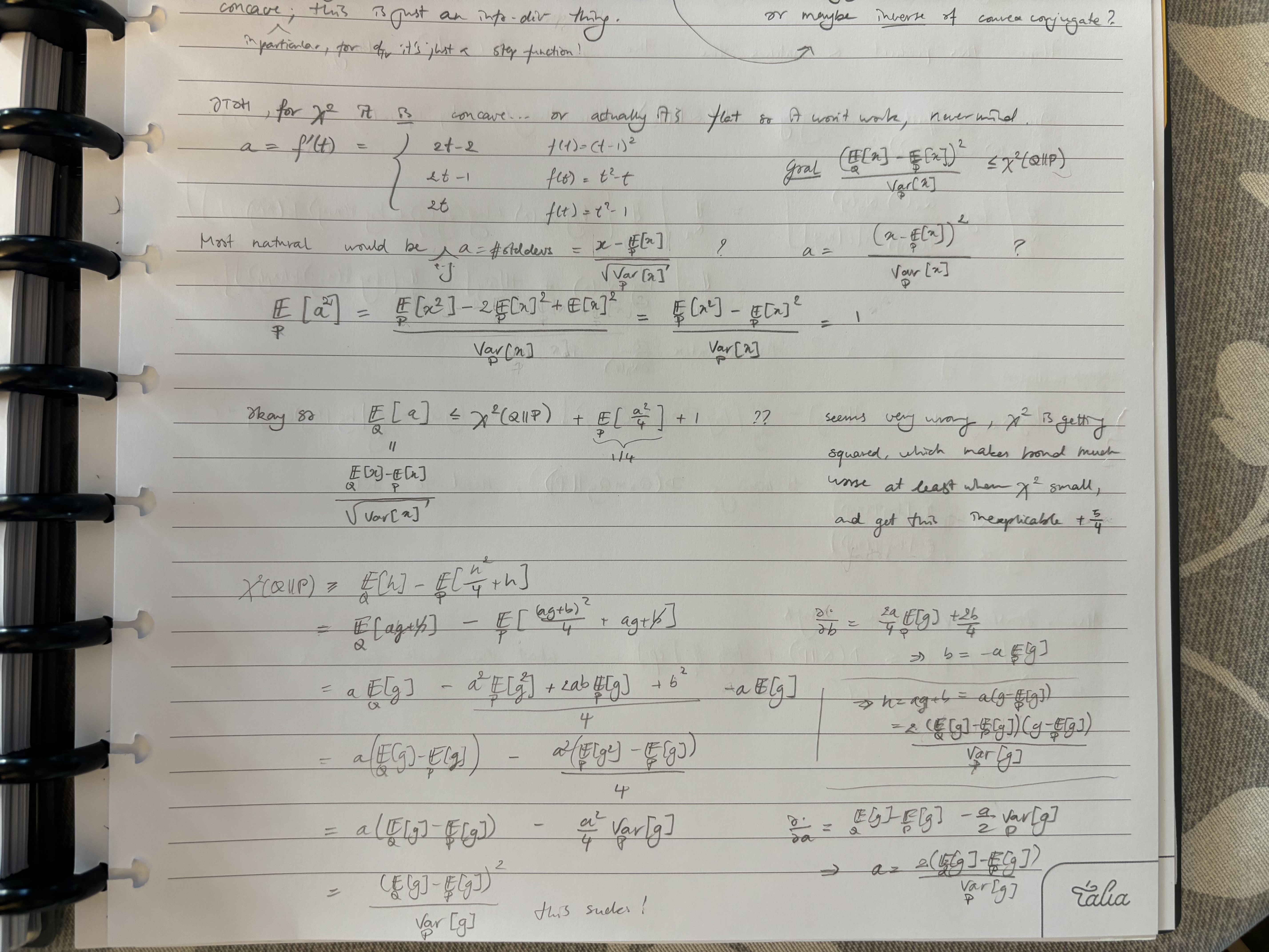
#to-think is something like $\E_{Q}[\Ba]^2 \le \chi^2\pff{Q}{P}\E_{P}[\Ba^2]$ true?
- then let $a(\Bx) \ce b(\Bx) - \E_P[b(\Bx)]$, giving
- $\LHS = \E_{\Bx \sim Q}\b{a(\Bx)}^2 = \E_{\Bx \sim Q}\b{b(\Bx)-\E_{\Bx' \sim P}\b{\Bx'}}^2 = \p{\E_Q\b{b(\Bx)}-\E_P\b{b(\Bx)}}^2$
- $\RHS = \E_{\Bx \sim P}\b{b(\Bx) - \E_{\Bx' \sim P}[b(\Bx')]} = \Var\b{b(\Bx)}$
- ok nice that sounds very promising actually
- and it suggests that a multiplicative version is cleaner in many cases?
As concentration bounds
These variational representations are in a sense a generalization of concentration bounds. Instead of only bounding the probability that $\Ba$ exceeds a certain value, they bound $\E_Q[\Ba]$ over any distribution $Q$ that is not too far from the prior $P$.
Formally, if we want to bound $p \ce \Pr_{P}[\Ba \ge v]$ for some threshold $v$, we can let $Q$ be the conditional distribution $\at{P}{\cdot \ge v}$, which makes $D^f\pff{Q}{P}$ a (decreasing) function of $p$, and write
\[
\al{
D^f \pff{Q}{P}
&\ge \E_{Q}\b{\Ba} - \E_{P}\b{f^*(\Ba)}\\
&= \E_{P}\bco{\Ba}{\Ba\ge v} - \E_{P}\b{f^*(\Ba)}\\
&\ge v - \E_{P}\b{f^*(\Ba)},
}
\]
which then gives an upper bound on $p$.
We have
\[
\al{
\log \f1p
&= \D\pff{Q}{P}\\
&\ge sv - \ln\E_{P}\b{e^{s\Ba}},
}
\]
that is, for $\Ba \sim P$,
\[
\Pr[\Ba \ge v] \le \f{\E\b{e^{s\Ba}}}{e^{sv}},
\]
which is the moment-generating function method (also known as Chernoff bound).
$\chi^2$-divergence
Let
\[
\al{
\mu &\ce \E_{P}[\Ba]\\
\sigma^2 &\ce \Var_{P}[\Ba]
}
\]
and let’s rewrite $v$ as $\mu + t\sigma$ for $t \ge 0$. Then we have
\[
\al{
\f1p - 1
&= \chi^2\pff{Q}{P}\\
&\ge \f{\p{\E_{Q}[\Ba]-\E_{P}[\Ba]}^2}{\Var_{P}[\Ba]}\\
&\ge \f{\p{v-\mu}^2}{\sigma^2}\\
&= t^2,
}
\]
that is, for $\Ba \sim P$,
\[
\Pr[\Ba \ge \mu + t\sigma] \le \f{1}{1+t^2},
\]
which is Chebyshev’s inequality.
Total variation distance
This one requires a bit more adaptation (and because of this is perhaps more of a hairpull). We have
\[
\al{
1-p
&= \dTV(P,Q)\\
&\ge \E_{x \sim Q}[a(x)] - \E_{x \sim P}[a(x)],
}
\]
but this only holds if $a(x) \in [0,1]$. So we perform the change of variables
\[
a(x) \gets \f{\min(a(x), v)}{v},
\]
which means that for any $\Ba \ge 0$ we have
\[
\al{
1-p
&\ge \E_{Q}\b{\f{\min(\Ba, v)}v} - \E_{P}\b{\f{\min(\Ba, v)}v}\\
&= 1 - \f{\E_{P}\b{\min(\Ba, v)}}v\\
&\ge 1 - \f{\E_{P}\b{\Ba}}v,
}
\]
so for $\Ba \sim P$,
\[
\Pr[\Ba \ge v] \le \f{\E[\Ba]}{v},
\]
which is Markov’s inequality.
See also
#to-think are most/all of these basically versions of Hölder’s inequality, the same way that Cauchy–Schwarz inequality can be understood in terms of weighting one sequence by the other? see SRLL p.128